Deep Learning from First Principles

— A systems-level journey through tensors and memory in Rust

• Prologue — Opening the Black Box
  • What We’ll Build
  • Who This Guide Is For (and Who It Is Not)
  • How to Use This Guide
  • Prerequisites and Philosophy
  • The Road Ahead
• The Tensor: From Math to Memory
  • Journey from Scalars to Tensors
  • Matrix Notation and Indexing
  • Design and Memory Layout
  • Implementation
  • Verifying Tensors
  • Visualizing the Memory in Math Format
  • Checkpoint: The Mental Leap
• Basic Tensor Arithmetic
  • The Element Wise Foundation
  • Implementation
  • Beyond Neighbors: The Road to Connectivity
• Linear Transformations and Aggregations
  • Transpose
    • Vector Transpose
    • Matrix Transpose
    • Implementation
  • Reduction
    • Implementation
  • Dot Product
    • Vector Vector Dot Product
    • Matrix Vector Dot Product
    • Matrix Matrix Dot Product
    • Implementation
  • Checkpoint
• Linear Regression
  • The Random Starting Point
  • The Loss Function
  • Optimizer
    • The Limits of Manual Tuning
    • Gradient Descent: Calculus Guided Tuning
  • Success: The Machine Learns
• Matrix Multiplication Revisited: The Need for Speed
  • The Bottleneck: Why Naive is Slow
  • The Evolution: From Loops to Iterators
  • Benchmark: The Reality of Optimization
  • Checkpoint
• Neural Network
  • Activation Function
    • Implementing Activation
  • Backward Pass
    • Implementing Single Layer Perceptron
  • Sigmoid Activation & BCE Loss
    • Sigmoid
    • Sigmoid BCE Shortcut
  • Limitation of Single Layer Perceptron
  • Multi Layer Perceptron
  • Implementation
  • Hyperparameter Tuning
  • Two Moons Experiment
  • Checkpoint
• Image Reconstruction: From Data to Geometry
  • The Portable BitMap (PBM)
  • The PBM Reader
  • The Tanh Activation Function
  • The Feature Scaling
  • Network Architecture
  • Thermal Overload
  • The Release Build
  • Conclustion
• Appendix A
• Appendix B
• Appendix C — Visualization and Auxiliary Tools

Prologue — Opening the Black Box

Modern machine learning tools have become remarkably easy to use and increasingly difficult to understand.

Most tutorials follow a similar path: introduce NumPy, then move to frameworks such as scikit‑learn, PyTorch, or TensorFlow. With only a few imports and function calls, you start training a model.

These are powerful tools, providing abstraction over multiple memory accesses, index mapping, numeric computations and assumptions - none of which are visible to users. Models work; gradients flow; machines learn. Yet the machinery underneath fades into abstraction.

This guide is an attempt to reverse that process. We build a minimal machine learning engine from first principles, exposing every step along the way. This guide exists because backpropagation is not confusing due to calculus, but because gradient flow is invisible in most learning resources.

Please note, we are not building a drop‑in replacement for PyTorch or ndarray.

The goal is not performance.

The goal is understanding.

What We’ll Build

This guide is a systems-level, hands-on guide to implementing the core machinery of machine learning in Rust. Step by step, we construct tensors, define matrix operations, implement backpropagation, and assemble a minimal neural network—using nothing more than the Rust standard library.

By the end, you will have built a small but complete deep learning engine and you will have developed a concrete mental model of how modern frameworks operate beneath their APIs.

If you are curious what the final system looks like, you can run it today. To run it on your system:

1. You need the Rust toolchain - rustup
2. Clone this repository - Build Your Own Neural Network
3. Run a release version - $ cargo run --release
4. Follow the instructions on screen

warning

If you choose Image Reconstruction example, it will take a long time to train depending on your machine’s architecture.

Who This Guide Is For (and Who It Is Not)

This guide is written for the curious readers who want to go beneath the surface.

It is for those who want to gain a deeper understanding of how tensors are represented in memory, how matrix multiplications are executed on hardware and how gradients actually flow through the data structures. In a nutshell, you will understand how a stream of $0$s and $1$s makes machines learn. It assumes you are comfortable reading code and willing to reason carefully about both mathematics and machines.

It is especially suited for:

• Software developers who want to understand neural networks beyond high-level APIs

• Readers learning Rust who want a demanding, systems-oriented project

It is not written for readers looking for a conceptual overview without implementation, for those seeking production-grade performance, or for complete beginners to programming or mathematics.

How to Use This Guide

The chapters are meant to be read sequentially. Each concept builds directly on the ones before it.

You are encouraged to:

• Take a pause when necessary
• Re-derive the math on your own
• Write the code yourself
• Experiment with the tool provided at each major section

Optionally:

• While using the visualizer tools, I encourage you to pause and verify the underlying data

This guide rewards patience. Do not rush. It is designed for depth, not speed.

Prerequisites and Philosophy

You do not need a formal background in linear algebra. Every mathematical concept used in this guide is derived as needed. You do need basic familiarity with Rust; enough to understand structs, enums, ownership, borrowing, module system and how to run tests with Cargo.

We use Rust not because it is the only way, but because its demand for explicitness makes it the perfect lens for viewing machine memory.

Beyond that, the philosophy is simple:

• Radical transparency: no hidden crates, no magic

• Clarity over ergonomics: explicit code beats elegant APIs

• Minimalism: one dependency—the Rust standard library, everything else we’ll build

If something works, you should be able to explain why it works.

The Road Ahead

We start with cargo new and we start building struct by struct, impl by impl. Afterwards, we compose these small pieces into layers and then connect them to build neural networks. We train them with different datasets.

We complete this guide by putting it all together, we build a network to reconstruct a small monochrome image at a higher resolution

assets/spiral_50.pbm:50 * 50 Original Image, assets/arrow.pbm, output/reconstructed_final.pbm:200*200 Reconstructed Image

And that’s where the story begins…

The Tensor: From Math to Memory

To build a neural network from scratch, we need to construct its foundational building block first. Any machine learning library performs the operations on a data structure known as Tensor. We will also build our own tensor.

Chapter Goals

• Develop the Intuition: Trace the journey from a single number to multi-dimensional data structures.
• Bridge the Gap: Map abstract mathematical notation (Ai,j​) to physical RAM addresses.
• Implement the Core: Build a Tensor struct in Rust that avoids the “pointer-chasing” performance traps of nested vectors.
• Visualize the Data: Create a formatting engine to inspect our matrices in a human-readable way.

Journey from Scalars to Tensors

Before typing a single line of code, we’ll share a mental model of the data structure. Tensors are categorized by their Rank, which simply describes the number of dimensions it has.

• Scalar (Rank 0): A single number (e.g. 5.3), used in day-to-day calculations. In code, this is a single variable like x = 5.3.
• Vector (Rank 1): When we arrange a collection of numbers in a linear fashion, we get a Vector. In code, this is represented as a flat array or Vec like a = [1.0, 2.0, 3.0]
• Matrix (Rank 2): When we stack multiple vectors together, we get a Matrix. In code, this would be an array of arrays (or Vec of Vecs): a = [[1.0, 2.0], [3.0, 4.0]]. Our workspace revolves around this.
• Tensor: When we arrange multiple matrices in an array or Vec, we get higher rank tensors. This would be beyond our scope in this guide and we will keep things simple by restricting ourselves up to 2D tensors only.

Here is a visual representation of the concept:

\[\begin{array}{ccc} \mathbf{Scalar} & \mathbf{Vector} & \mathbf{Matrix} \\ \color{#E74C3C}{1} & \left[\begin{matrix} \color{cyan}1 \\ \color{cyan}2 \end{matrix} \right] & \left[\begin{matrix} \color{magenta}{1} & \color{magenta}{2} \\\ \color{magenta}{3} & \color{magenta}{4} \end{matrix} \right] \end{array}\]

While tensors can theoretically have infinite rank, we will focus our engine on Rank 2 (Matrices) to keep our implementation lean and easy to understand.

Matrix Notation and Indexing

In mathematics, a matrix $A$ with $m$ rows and $n$ columns is referred to as an $m \times n$ matrix. We identify an individual element within that matrix using subscripts $A_{i,j}$

Where:

• i is the row index (1 ≤ i ≤ m)
• j is the column index (1 ≤ j ≤ n)

In code, we usually achieve this by indexing into the array:

a = [[1, 2], [3, 4]];
println!("{}", a[0][0]); // Output: 1

Note on Indexing: Mathematics typically uses 1-based indexing $(1…n)$, while Rust uses 0-based indexing (0...n−1). Throughout this guide, our code will always follow the 0-based programming convention.

Design and Memory Layout

With the mathematical background, now we’ll design our Tensor. We need a fast, flexible and easy to index data structure to store multiple data points.

An array matches most of our requirements but Rust arrays can’t grow or shrink dynamically at run time.

To maintain flexibility, we’ll use Vec instead. A naive Rust implementation may look like this: Vec<Vec<f32>>. However, that won’t be an efficient design for two reasons:

1. Indirection (Pointer Chasing): A Vec of Vec is a very performance-intensive structure. Each inner Vec is a separate allocation on the heap. Accessing elements requires jumping to different memory locations.

   \[\begin{array}{c|l} \text{Outer Index} & \text{Pointer to Inner Vec} \\\\ \hline 0 & \color{#3498DB}{\rightarrow [v_{0,0}, v_{0,1}, v_{0,2}]} \\\\ 1 & \color{#E74C3C}{\rightarrow [v_{1,0}, v_{1,1}, v_{1,2}]} \\\\ 2 & \color{#2ECC71}{\rightarrow [v_{2,0}, v_{2,1}, v_{2,2}]} \\\\ \end{array}\]

2. Rigidity: Vec of Vec would permanently limit our application to a 2D matrix and reshape or transpose would be difficult to handle.

These costs are invisible at small scales but dominate performance and correctness as models grow.

Solution: Flat Buffer

Instead we will store all the numbers in a Vec, allowing cache locality for efficient access patterns, and keep a separate shape vector to guide us on how to interpret the flat list. We use this convention: shape[0] is number of rows and shape[1] is number of columns.

pub struct Tensor {
    data: Vec<f32>,
    shape: Vec<usize>,
}

If this design makes sense to you, you already understand how many tensor libraries store tensors.

Implementation

Let’s get our hands dirty and initialize the project:

$ cargo new build_your_own_nn

We’ll define our tensor and a custom error type TensorError in src/tensor.rs. We must define a few errors and handle them while working with tensors.

use std::error::Error;

#[derive(Debug, PartialEq)]
pub enum TensorError {
    ShapeMismatch,
    InvalidRank,
    InconsistentData,
}

impl Error for TensorError {}

impl std::fmt::Display for TensorError {
    fn fmt(&self, f: &mut std::fmt::Formatter<'_>) -> std::fmt::Result {
        match self {
            TensorError::ShapeMismatch => write!(f, "Tensor shapes do not match for the operation."),
            TensorError::InvalidRank => write!(f, "Tensor rank is invalid (must be 1D or 2D)."),
            TensorError::InconsistentData => write!(f, "Data length does not match tensor shape."),
        }
    }
}

pub struct Tensor {
    data: Vec<f32>,
    shape: Vec<usize>,
}

impl Tensor {
    pub fn new(data: Vec<f32>, shape: Vec<usize>) -> Result<Tensor, TensorError> {
        todo!()
    }

    pub fn data(&self) -> &[f32] {
        todo!()
    }

    pub fn shape(&self) -> &[usize] {
        todo!()
    }
}

To make this accessible, we expose the module in src/lib.rs:

pub mod tensor;

Verifying Tensors

Tensors are at the heart of our engine. We’ll follow a Test Driven Development approach for our Tensor. This ensures our thinking around the tensors and every time we make a change, we ensure we are not breaking the core.

We will place our tests in a dedicated tests/ directory at the root of the project. This treats our library as an external crate, exactly how a user would interact with it.

Create a file at tests/test_tensor.rs:

use build_your_own_nn::tensor::Tensor;
use build_your_own_nn::tensor::TensorError;

#[cfg(test)]
mod tests {
    use super::*;

    // The happy path test
    #[test]
    fn test_tensor_creation() {
        let data = vec![1.0, 2.0, 3.0, 4.0];
        let shape = vec![2, 2];
        let tensor = Tensor::new(data.clone(), shape.clone()).unwrap();

        assert_eq!(tensor.data(), &data);
        assert_eq!(tensor.shape(), &shape);
    }

    // Test the invariant; ensure data and shape are consistent with each other
    #[test]
    fn test_invalid_shape_creation() {
        let result = Tensor::new(vec![1.0], vec![2, 2]);
        assert!(result.is_err());
        assert_eq!(result.unwrap_err(), TensorError::InconsistentData);
    }

    // To test our self imposed restriction of allowing only up to 2D
    // When we'll allow more dimensions, this test should be removed
    #[test]
    fn test_rank_limits() {
        // We currently don't support 3D tensors (Rank 3)
        let result = Tensor::new(vec![1.0; 8], vec![2, 2, 2]);

        assert!(result.is_err());
        assert_eq!(result.unwrap_err(), TensorError::InvalidRank);
    }
}

The tests will fail if we run cargo test. Now, let’s replace those placeholders with our logic in tensor.rs:

impl Tensor {
    pub fn new(data: Vec<f32>, shape: Vec<usize>) -> Result<Tensor, TensorError> {
        if shape.len() == 0 || shape.len() > 2 {
            return Err(TensorError::InvalidRank);
        }

        if data.len() != shape.iter().product::<usize>() {
            return Err(TensorError::InconsistentData);
        }
        Ok(Tensor { data, shape })
    }

    pub fn data(&self) -> &[f32] {
        &self.data
    }

    pub fn shape(&self) -> &[usize] {
        &self.shape
    }
}

Now, if we run the tests, we can see the tests passing.

$ cargo test
...

     Running tests/test_tensor.rs (target/debug/deps/test_tensor-25b5f99a2a90f9bb)

test tests::test_tensor_creation ... ok
test tests::test_invalid_shape_creation ... ok
test tests::test_rank_limits ... ok

NOTE

We will be using standard Rust module system throughout.

Currently the directory structure should look like the following:

src
├── lib.rs
├── main.rs
└── tensor.rs
tests
└── test_tensor.rs
Cargo.toml

Visualizing the Memory in Math Format

TIP

This section is optional but highly recommended.

You may skip it without losing any conceptual understanding in later chapters; the only difference will be how easily you can visualize tensor data during debugging and exploration.

The definition and implementation of the tensor are now clear. We now need a way to intuitively inspect the data. Inspecting a Vec of floating-point numbers in a single line is not very helpful for 2D data.

To fix this, we will implement the std::fmt::Display trait for our Tensor. This will allow us to print tensors in a recognizable matrix format and ensure our understanding of one dimensional data to $2D$ matrix transformation.

Visualization Rules

1. 1D (Vector): We’ll use the default debug format (e.g., [1.0, 2.0, 3.0]).

2. 2D (Matrix): We’ll use the Row-Major convention $(row \times cols + col)$ to pick elements and wrap them in a grid.

   Let’s take an example,

   \[\begin{bmatrix} \color{cyan}1_{0} & \color{magenta}2_{1} & \color{#2ECC71}3_{2} & \color{#D4A017}4_{3} \end{bmatrix} \implies \begin{bmatrix} \color{cyan}1_{(0)} & \color{magenta}2_{(1)} \\\ \color{#2ECC71}3_{(2)} & \color{#D4A017}4_{(3)} \end{bmatrix}\]

   Here, we have a Vec of length 4 with 2 rows and 2 columns. The first row is formed by the elements at index 0 and index 1 and the second row is formed by the elements at index 2 and index 3.

3. We’ll output only up to four decimal points ensuring uniformity and alignment

Based on these intuitions, we first write the tests:

#[test]
fn test_tensor_display_2d() -> Result<(), TensorError> {
    let tensor = Tensor::new(vec![1.0, 2.0, 3.0, 4.0], vec![2, 2])?;

    let output = format!("{}", tensor);

    println!("{}", output);

    assert!(output.contains("|  1.0000,   2.0000|"));
    assert!(output.contains("|  3.0000,   4.0000|"));
}

#[test]
fn test_tensor_display_alignment() -> Result<(), TensorError> {
    let tensor = Tensor::new(vec![1.23456, 2.0, 100.1, 0.00001], vec![2, 2])?;

    let output = format!("{}", tensor);

    assert!(output.contains("  1.2346"));
    assert!(output.contains("  0.0000"));
}

#[test]
fn test_tensor_display_1d() -> Result<(), TensorError> {
    let tensor = Tensor::new(vec![1.0, 2.0, 3.0], vec![3])?;

    let output = format!("{}", tensor);
    assert!(output.contains("[1.0, 2.0, 3.0]"));
}

Then we implement the Display trait for our Tensor:

impl std::fmt::Display for Tensor {
    fn fmt(&self, f: &mut std::fmt::Formatter<'_>) -> std::fmt::Result {
        // Use default debug format for 1D vectors
        if self.shape.len() != 2 {
            return write!(f, "{:?}", self.data);
        }

        let rows = self.shape[0];
        let cols = self.shape[1];

        for row in 0..rows {
            write!(f, "  |")?;
            for col in 0..cols {
                let index = row * cols + col;
                write!(f, "{:>8.4}", self.data[index])?;

                if col < cols - 1 {
                    write!(f, ", ")?;
                }
            }
            writeln!(f, "|")?;
        }
        Ok(())
    }
}

Finally, we see it in action:

use build_your_own_nn::tensor::{Tensor, TensorError};

fn main() -> Result<(), TensorError> {
    // One dimensional vector
    let v = Tensor::new(vec![1.0, 2.0, 3.0, 4.0], vec![4]).unwrap();

    // Two dimensional 2 * 2 Matrix
    let a = Tensor::new(vec![1.0, 2.0, 3.0, 4.0], vec![2, 2]).unwrap();

    // Two dimensional 3 * 3 Matrix
    let b = Tensor::new(
        vec![1.0, 2.0, 3.0, 4.0, 5.0, 6.0, 7.0, 8.0, 9.0],
        vec![3, 3],
    ).unwrap();

    println!("1D Vector: \n{}", v);

    println!("2D 2*2: \n{}", a);

    println!("2D 3*3 \n{}", b);
}

1D Vector: 
[1.0, 2.0, 3.0, 4.0]
2D 2*2: 
  |  1.0000,   2.0000|
  |  3.0000,   4.0000|

2D 3*3 
  |  1.0000,   2.0000,   3.0000|
  |  4.0000,   5.0000,   6.0000|
  |  7.0000,   8.0000,   9.0000|

Challenge: Personalize Your Visualization

The formatting we implemented is just one way to view the data. Designing a clear visualization is a great way to deepen your understanding of the underlying structure. I encourage you to experiment with your own Display implementation.

For instance, could you add row/column headers? Or perhaps truncate very large matrices so they don’t overwhelm your terminal? There is no correct style. There is only the one that helps you debug your neural network most effectively.

Checkpoint: The Mental Leap

You have reached a critical milestone. By implementing the Display trait, you’ve moved beyond treating data as an abstract list and started treating it as a geometric structure.

If you understand how the formula $(row×cols)+col$ folds a flat buffer into a $2D$ grid, you have mastered the foundational logic of all modern machine learning.

A tensor that can only be stored is not very useful. Learning systems require tensors to interact: values must be added, scaled, and transformed. Before we can build models, we need a minimal algebra.

Basic Tensor Arithmetic

If you already have a good grasp of tensor arithmetic and linear algebra, you may skip to Linear Regression.

Moving to the next phase of our journey, we step into the machinery of movement: Basic Tensor Arithmetic. If tensors are the bones of our system, operations are muscles. In this chapter, we transition from merely storing data to transforming it. We begin with the most intuitive operations—element wise arithmetic.

The Element Wise Foundation

We treat matrices as dynamic containers. For the most basic operations - Addition, Subtraction, Multiplication (the Hadamard Product) and Division—we follow a strict rule: the matrices must be of identical shape. We don’t just operate on numbers; we operate on neighborhoods.

Mathematically, if $A$ and $B$ are both $m \times n$, then any operation $g$ on $A$ and $B$ is defined as:

\[C_{i,j}​=g(A_{i,j}​, B_{i,j}​)\]

where $g$ is either $+$, $-$, $\odot$ or $\oslash$.

Thus we get the following,

\[\begin{bmatrix} \color{cyan}{1} & \color{magenta}2 \\\ \color{#D4A017}3 & \color{#2ECC71}4 \end{bmatrix} + \begin{bmatrix} \color{cyan}5 & \color{magenta}6 \\\ \color{#D4A017}7 & \color{#2ECC71}8 \end{bmatrix} = \begin{bmatrix} \color{cyan} 1 + 5 & \color{magenta} 2+6 \\\ \color{#D4A017}3 + 7 & \color{#2ECC71}4 + 8 \end{bmatrix} = \begin{bmatrix} \color{cyan}6 & \color{magenta}8 \\\ \color{#D4A017}10 & \color{#2ECC71}12 \end{bmatrix}\] \[\begin{bmatrix} \color{cyan}{5} & \color{magenta}6 \\\ \color{#D4A017}7 & \color{#2ECC71}8 \end{bmatrix} - \begin{bmatrix} \color{cyan}1 & \color{magenta}2 \\\ \color{#D4A017}3 & \color{#2ECC71}4 \end{bmatrix} = \begin{bmatrix} \color{cyan} 5 - 1 & \color{magenta} 6 - 2\\\ \color{#D4A017} 7 - 3 & \color{#2ECC71} 8 - 4 \end{bmatrix} = \begin{bmatrix} \color{cyan}4 & \color{magenta}4\\\ \color{#D4A017}4 & \color{#2ECC71}4 \end{bmatrix}\] \[\begin{bmatrix} \color{cyan}{1} & \color{magenta}2 \\\ \color{#D4A017}3 & \color{#2ECC71}4 \end{bmatrix} \odot \begin{bmatrix} \color{cyan}5 & \color{magenta}6 \\\ \color{#D4A017}7 & \color{#2ECC71}8 \end{bmatrix} = \begin{bmatrix} \color{cyan}1 \cdot 5 & \color{magenta}2 \cdot 6\\\ \color{#D4A017}3 \cdot 7 & \color{#2ECC71}4 \cdot 8 \end{bmatrix} = \begin{bmatrix} \color{cyan}5 & \color{magenta}12\\\ \color{#D4A017}21 & \color{#2ECC71}32 \end{bmatrix}\] \[\begin{bmatrix} \color{cyan}{1} & \color{magenta}2 \\\ \color{#D4A017}3 & \color{#2ECC71}4 \end{bmatrix} \oslash \begin{bmatrix} \color{cyan}5 & \color{magenta}6 \\\ \color{#D4A017}7 & \color{#2ECC71}8 \end{bmatrix} = \begin{bmatrix} \color{cyan} \frac{1} {5} & \color{magenta}\frac{2}{6}\\\ \color{#D4A017}\frac{3}{7} & \color{#2ECC71}\frac{4}{8} \end{bmatrix} = \begin{bmatrix} \color{cyan}0.2000 & \color{magenta}0.3333\\\ \color{#D4A017}0.4286 & \color{#2ECC71}0.5000 \end{bmatrix}\]

We have the mathematical blueprint, let’s translate these concepts into Rust code.

Implementation

We should expose methods for add, sub, mul and div. We’ll first add these method definitions into our existing tensor impl block.

    pub fn add(&self, other: &Tensor) -> Result<Tensor, TensorError> {
        todo!()
    }

    pub fn sub(&self, other: &Tensor) -> Result<Tensor, TensorError> {
        todo!()
    }

    pub fn mul(&self, other: &Tensor) -> Result<Tensor, TensorError> {
        todo!()
    }

    pub fn div(&self, other: &Tensor) -> Result<Tensor, TensorError> {
        todo!()
    }

Now we’ll write tests for these methods:

#[test]
pub fn test_tensor_operations() -> Result<(), TensorError>  {
    use std::vec;

    let a = Tensor::new(vec![1.0, 2.0, 3.0, 4.0], vec![2, 2])?;
    let b = Tensor::new(vec![5.0, 6.0, 7.0, 8.0], vec![2, 2])?;

    let c = a.add(&b)?;
    assert_eq!(c.data(), &[6.0, 8.0, 10.0, 12.0]);
    assert_eq!(c.shape(), &[2, 2]);

    let d = a.sub(&b)?;
    assert_eq!(d.data(), &[-4.0, -4.0, -4.0, -4.0]);
    assert_eq!(d.shape(), &[2, 2]);

    let e = a.mul(&b)?;
    assert_eq!(e.data(), &[5.0, 12.0, 21.0, 32.0]);
    assert_eq!(e.shape(), &[2, 2]);

    let f = a.div(&b)?;
    let epsilon = 1e-4;
    for (l, r) in f.data().iter().zip([0.2000, 0.3333, 0.4286, 0.5000].iter()) {
        assert!(
            (l - r).abs() < epsilon,
            "Values {} and {} are not close enough",
            l,
            r
        );
    }
}

The tests need concrete implementations to pass. We will add a common method inside the impl block and use it to unify all the element wise operations using function pointers:

    fn _element_wise_op(
        &self,
        other: &Tensor,
        op: impl Fn(f32, f32) -> f32,
    ) -> Result<Tensor, TensorError> {
        if self.shape != other.shape {
            return Err(TensorError::ShapeMismatch);
        }

        let data: Vec<f32> = self
            .data
            .iter()
            .zip(other.data.iter())
            .map(|(&a, &b)| op(a, b))
            .collect();

        Tensor::new(data, self.shape.clone())
    }

    pub fn add(&self, other: &Tensor) -> Result<Tensor, TensorError> {
        self._element_wise_op(other, |a, b| a + b)
    }

    pub fn sub(&self, other: &Tensor) -> Result<Tensor, TensorError> {
        self._element_wise_op(other, |a, b| a - b)
    }

    pub fn mul(&self, other: &Tensor) -> Result<Tensor, TensorError> {
        self._element_wise_op(other, |a, b| a * b)
    }

    pub fn div(&self, other: &Tensor) -> Result<Tensor, TensorError> {
        self._element_wise_op(other, |a, b| a / b)
    }

Let’s end this chapter by visualizing the result exactly we have defined the operations:

fn main() {
    let a = Tensor::new(vec![1.0, 2.0, 3.0, 4.0], vec![2, 2]).unwrap();
    let b = Tensor::new(vec![5.0, 6.0, 7.0, 8.0], vec![2, 2]).unwrap();

    println!("Matrix A:\n{a}");
    println!("Matrix B:\n{b}");

    println!("A + B\n{}", a.add(&b).unwrap());
    println!("A - B\n{}", a.sub(&b).unwrap());
    println!("A ☉ B\n{}", a.mul(&b).unwrap());
    println!("A ø B\n{}", a.div(&b).unwrap());
}

Matrix A:
  |  1.0000,   2.0000|
  |  3.0000,   4.0000|

Matrix B:
  |  5.0000,   6.0000|
  |  7.0000,   8.0000|

A + B
  |  6.0000,   8.0000|
  | 10.0000,  12.0000|

A - B
  | -4.0000,  -4.0000|
  | -4.0000,  -4.0000|

A ☉ B
  |  5.0000,  12.0000|
  | 21.0000,  32.0000|

A ø B
  |  0.2000,   0.3333|
  |  0.4286,   0.5000|

Beyond Neighbors: The Road to Connectivity

We have mastered element wise arithmetic, where tensors interact only with their mirror images in the opposing container. For a neural network to identify a pattern though, it must be able to look across, not just its mirror match.

In the next chapter, we introduce the operations that enable this global view. We will learn to flip our perspective with Transpose, condense our knowledge with Sum, and finally, implement Matrix Multiplication: the engine’s heart.

Linear Transformations and Aggregations

Previously, we treated matrices as containers, adding or multiplying elements in the same neighborhood. To build a neural network, we need operations that move data across different neighborhoods.

Chapter Goals

By the end of this section, you will have implemented:

• Spatial Reorientation (Transpose): Mastering the “Index Swap” logic to flip tensors between row-major and column-major perspectives.
• Information Compression (Reduction): Implementing axis-based summation (Axis 0 vs. Axis 1) to extract global or feature-specific totals.
• The Computational Workhorse (Dot Product): Developing a naive $O(n^3)$ matrix multiplication engine that handles vector-vector, matrix-vector, and matrix-matrix interactions.

Why This Matters for Machine Learning

In a typical neural network “forward pass,” these operations are the primary actors:

• Dot Products allow input features to interact with learned weights.
• Transpositions are essential for aligning data during backpropagation.
• Reductions are the foundation for calculating loss and cost functions.

Below are the three operations we’ll need for Machine Learning.

Transpose

The Transpose operation changes the orientation of a matrix: rows become columns, and columns become rows. Mathematically, this is expressed as:

\[(A^T​)_{\color{cyan}{i},\color{magenta}{j}}=A_{\color{magenta}{j},\color{cyan}{i}}​\]

Vector Transpose

\[\begin{bmatrix} \color{cyan}{1} & \color{magenta}{2} & \color{gold}{3} & \color{lime}{4} \end{bmatrix} \xrightarrow{transpose} \begin{bmatrix} \color{cyan}{1} \\\ \color{magenta}{2} \\\ \color{gold}{3} \\\ \color{lime}{4} \end{bmatrix}\]

Matrix Transpose

\[\begin{bmatrix} \color{cyan}{1} & \color{cyan}{2} \\\ \color{magenta}{3} & \color{magenta}{4} \\\ \color{gold}{5} & \color{gold}{6}\end{bmatrix} \xrightarrow{transpose} \begin{bmatrix} \color{cyan}{1} & \color{magenta}{3} & \color{gold}{5} \\\ \color{cyan}{2} & \color{magenta}{4} & \color{gold}{6} \end{bmatrix}\]

Implementation

With this mathematical background, we can now understand how the transpose operation will transform the data. Based on the understanding, we start writing the tests and implement the operation:

    #[test]
    fn test_transpose_square() -> Result<(), TensorError> {
        // 1.0, 2.0

        // 3.0, 4.0

        let a = Tensor::new(vec![1.0, 2.0, 3.0, 4.0], vec![2, 2])?;

        let swapped = a.transpose()?;

        // Should become:

        // 1.0, 3.0

        // 2.0, 4.0

        assert_eq!(swapped.data(), &[1.0, 3.0, 2.0, 4.0]);

        assert_eq!(swapped.shape(), &[2, 2]);
        Ok(())
    }

    

    #[test]
    fn test_transpose_rectangular() -> Result<(), TensorError> {
        let a = Tensor::new(vec![1.0, 2.0, 3.0, 4.0, 5.0, 6.0], vec![2, 3])?;
        let swapped = a.transpose()?;

        assert_eq!(swapped.data(), &[1.0, 4.0, 2.0, 5.0, 3.0, 6.0]);

        // The row, column should be reversed
        assert_eq!(swapped.shape(), &[3, 2]);
        Ok(())
    }

    #[test]
    fn test_transpose_1d() -> Result<(), TensorError> {
        let a = Tensor::new(vec![1.0, 2.0, 3.0, 4.0, 5.0, 6.0], vec![6])?;
        let swapped = a.transpose()?;

        // No change for 1D
        assert_eq!(swapped.data(), &[1.0, 2.0, 3.0, 4.0, 5.0, 6.0]);
        assert_eq!(swapped.shape(), &[6]);
        Ok(())
    }

To transpose matrices in Rust, we physically rebuild the data in a new Vec. While some libraries use “strides” (metadata changes), rebuilding keeps our memory contiguous, which makes subsequent operations faster for the CPU to predict.

The Logic:

1. Check the Rank: We only support transposing 1D or 2D tensors.

2. The 1D Shortcut: In a 1D vector, there’s no “grid” to flip and we simply return a copy.

3. The 2D Re-map: We use Index Swap. In the original data, we find an element at $row * cols + col$. In transposed data, the position becomes $col * rows + row$.

    pub fn transpose(&self) -> Result<Tensor, TensorError> {
        if self.shape.len() != 1 && self.shape.len() != 2 {
            return Err(TensorError::InvalidRank);
        }

        if self.shape.len() == 1 {
            return Tensor::new(self.data.clone(), self.shape.clone());
        }

        let rows = self.shape[0];
        let cols = self.shape[1];
        let mut transposed_data = vec![0.0; self.data.len()];

        for row in 0..rows {
            for col in 0..cols {
                transposed_data[col * rows + row] = self.data[row * cols + col];
            }
        }

        Tensor::new(transposed_data, vec![cols, rows])
    }

Reduction

A matrix or a vector gives us information about individual elements, but we often need an aggregation of those individual elements. There are three types of aggregation we can perform row wise total (axis 1 sum) or column wise total (axis 0 sum) or grand total where the whole matrix reduces to a single scalar.

Consider a matrix representing car sales over three months:

\[\begin{array}{c|ccc|c} \mathbf {} & \mathbf{Maruti} & \mathbf{Hyundai} & \mathbf{Toyota} & \mathbf{Row\ Wise\ Total} \\ \hline Oct & 1000 & 2000 & 3000 & \color{gold}{6000} \\ Nov & 1200 & 1800 & 2000 & \color{gold}{5000} \\ Dec & 1500 & 2500 & 2200 & \color{gold}{6200} \\ \hline \mathbf{Column\ Wise\ Total} & \color{cyan}{3700} & \color{cyan}{6300} & \color{cyan}{7200} & \mathbf{\color{lime}17200\ (Grand\ Total)} \\ \end{array}\]

Implementation

Following our mathematical definition, let’s start defining our method first. We should be able to sum across rows or columns or reduce the whole tensor into a single scalar value. We would need the axis on which to sum but for a global sum, we don’t have anything to pass. We will use Option type for the axis parameter and we will return a tensor object.

Let’s put the definition in a function in the existing tensor impl

pub fn sum(&self, axis: Option<usize>) -> Result<Tensor, TensorError> {
    todo!()
}

We now have the definition ready, let’s start writing a few tests. The following set of tests should cover most of the cases.

fn setup_matrix_for_reduction() -> Tensor {
        let data = vec![
            1000.0, 2000.0, 3000.0, 1200.0, 1800.0, 2000.0, 1500.0, 2500.0, 2200.0,
        ];
        Tensor::new(data, vec![3, 3]).expect("Failed to create matrix for reduction tests")
    }

    #[test]
    fn test_reduce_sum_global() {
        let tensor = setup_matrix_for_reduction();
        let res = tensor.sum(None).unwrap();

        assert_eq!(res.data(), &[17200.0]);
        assert_eq!(res.shape(), &[1]);
    }

    #[test]
    fn test_reduce_sum_axis_0_total() {
        let tensor = setup_matrix_for_reduction();
        let res = tensor.sum(Some(0)).unwrap();

        assert_eq!(res.data(), &[3700.0, 6300.0, 7200.0]);
        assert_eq!(res.shape(), &[3]);
    }

    #[test]
    fn test_reduce_sum_axis_1_total() {
        let tensor = setup_matrix_for_reduction();
        let res = tensor.sum(Some(1)).unwrap();

        assert_eq!(res.data(), &[6000.0, 5000.0, 6200.0]);
        assert_eq!(res.shape(), &[3]);
    }

    #[test]
    fn test_reduce_sum_1d_tensor() {
        let tensor = Tensor::new(vec![1.0, 2.0, 3.0], vec![3]).unwrap();
        let res = tensor.sum(Some(0)).unwrap();

        assert_eq!(res.data(), &[6.0]);
        assert_eq!(res.shape(), &[1]);
    }

    #[test]
    fn test_reduce_sum_invalid_axis() {
        let tensor = setup_matrix_for_reduction();
        let res = tensor.sum(Some(2));

        assert_eq!(res.err(), Some(TensorError::InvalidRank));
    }

    #[test]
    fn test_reduce_sum_empty() {
        let tensor = Tensor::new(vec![], vec![0]).unwrap();
        let res = tensor.sum(Some(2));

        assert_eq!(res.err(), Some(TensorError::InvalidRank));
    }

Now let’s complete the implementation of reduction operation and run the tests

pub fn sum(&self, axis: Option<usize>) -> Result<Tensor, TensorError> {
        match axis {
            None => {
                let sum: f32 = self.data.iter().sum();
                Tensor::new(vec![sum], vec![1])
            }

            Some(0) => {
                if self.shape.len() < 2 {
                    return self.sum(None);
                }
                let rows = self.shape[0];
                let cols = self.shape[1];
                let mut result_data = vec![0.0; cols];

                for r in 0..rows {
                    for c in 0..cols {
                        result_data[c] += self.data[r * cols + c];
                    }
                }
                Tensor::new(result_data, vec![cols])
            }

            Some(1) => {
                if self.shape.len() < 2 {
                    return self.sum(None);
                }
                let rows = self.shape[0];
                let cols = self.shape[1];
                let mut result_data = vec![0.0; rows];

                for r in 0..rows {
                    for c in 0..cols {
                        result_data[r] += self.data[r * cols + c];
                    }
                }
                Tensor::new(result_data, vec![rows])
            }

            _ => Err(TensorError::InvalidRank),
        }
    }

Dot Product

Dot Product (a.k.a Matrix Multiplication or matmul) is the most critical operation for neural networks. Following our neighborhood analogy, this operation allows numbers to infer information across neighborhoods.

If this math is familiar, feel free to skim to the Rust implementation. The code is where the real learning happens.

We’ll go slowly over the concepts and examples, if required please re-read this topic until you get a good grasp. I recommend, practicing a few examples by hand too.

If this feels slow, that’s normal. This is the hardest operation we’ll implement by hand.

Vector Vector Dot Product

Mathematically, the dot product of two vectors $A$ and $B$ of length $n$ is defined as:

\[A \cdot B = \sum_{i=1}^{n} A_i \cdot B_i\]

Let’s look at an example:

\[\begin{bmatrix} \color{#2ECC71}{1} \\\ \color{cyan}{2} \\\ \color{magenta}{3} \\\ \color{#D4A017}{4} \end{bmatrix} \cdot \begin{bmatrix} \color{#2ECC71}1 \\\ \color{cyan}2 \\\ \color{magenta}3 \\\ \color{#D4A017}4 \end{bmatrix} = \color{#2ECC71}{(1 \times 1)} \color{white}+ \color{cyan}{(2 \times 2)} \color{white}+ \color{magenta}{(3 \times 3)} \color{white}+ \color{#D4A017}{(4 \times 4)}\color{white}=30\]

Matrix Vector Dot Product

In a Matrix Vector dot product, we calculate the dot product of every row from the matrix with the single column of the vector.

To perform a dot product between a matrix $A$ and a vector $v$, the number of columns in the matrix must equal the number of elements (rows) in the vector.

If matrix $A$ has the shape $(m \times n)$ and vector $v$ has the shape $(n \times 1)$, the resulting vector $w$ will have the shape $(m \times 1)$.

Matrix Vector dot product is defined as:

\[C_{m} = A_{m, :} \cdot v\]

Let’s take an example:

\[\begin{bmatrix} \color{#2ECC71}{1} & \color{#2ECC71}{2} & \color{#2ECC71}{3} \\\ \color{#D4A017}{4} & \color{#D4A017}{5} & \color{#D4A017}{6} \end{bmatrix} \cdot \begin{bmatrix} \color{cyan}{7} \\\ \color{cyan}{8} \\\ \color{cyan}{9} \end{bmatrix} = \begin{bmatrix} \color{#2ECC71}{[1, 2, 3]} \cdot \color{cyan}{[7, 8, 9]} \\\ \color{#D4A017}{[4, 5, 6]} \cdot \color{cyan}{[7, 8, 9]} \end{bmatrix} = \begin{bmatrix} (\color{#2ECC71}{1} \times \color{cyan}{7} + \color{#2ECC71}{2} \times \color{cyan}{8} + \color{#2ECC71}{3} \times \color{cyan}{9}) \\\ (\color{#D4A017}{4} \times \color{cyan}{7} + \color{#D4A017}{5} \times \color{cyan}{8} + \color{#D4A017}{6} \times \color{cyan}{9}) \end{bmatrix} = \begin{bmatrix} 50 \\\ 122 \end{bmatrix}\]

Matrix Matrix Dot Product

In a Matrix-Matrix dot product (often simply called Matrix Multiplication), we calculate the dot product of every row from the first matrix with every column of the second matrix.

To perform a dot product between matrix $A$ and matrix $B$, the number of columns in $A$ must match the number of rows in $B$.

If $A$ is $(m \times n)$ and $B$ is $(n \times p)$, the resulting matrix $C$ will have the shape $(m \times p)$.

Matrix Multiplication is defined as:

\[C_{m,p} = A_{m, :} \cdot B_{:, p}\]

Let’s take an example:

\[\begin{bmatrix} \color{#2ECC71}1 & \color{#2ECC71}2 & \color{#2ECC71}3 \\\ \color{#D4A017}4 & \color{#D4A017}5 & \color{#D4A017}6 \end{bmatrix} \cdot \begin{bmatrix} \color{cyan}7 & \color{magenta}8 \\\ \color{cyan}9 & \color{magenta}10 \\\ \color{cyan}11 & \color{magenta}12 \end{bmatrix} = \begin{bmatrix} \color{#2ECC71}{[1, 2, 3]} \cdot \color{cyan}{[7, 9, 11]} & \color{#2ECC71}{[1, 2, 3]}\cdot \color{magenta}{[8, 10, 12]} \\\ \color{#D4A017}[4, 5, 6] \cdot \color{cyan}{[7, 9, 11]} & \color{#D4A017}[4, 5, 6] \cdot \color{magenta}{[8, 10, 12]} \\\ \end{bmatrix} = \begin{bmatrix} (\color{#2ECC71}{1} \times \color{cyan}{7} + \color{#2ECC71}{2} \times \color{cyan}{9} + \color{#2ECC71}{3} \times \color{cyan}{11}) & (\color{#2ECC71}{1} \times \color{magenta}{8} + \color{#2ECC71}{2} \times \color{magenta}{10} + \color{#2ECC71}{3} \times \color{magenta}{12}) \\\ (\color{#D4A017}{4} \times \color{cyan}{7} + \color{#D4A017}{5} \times \color{cyan}{9} + \color{#D4A017}{6} \times \color{cyan}{11}) & (\color{#D4A017}{4} \times \color{magenta}{8} + \color{#D4A017}{5} \times \color{magenta}{10} + \color{#D4A017}{6} \times \color{magenta}{12}) \end{bmatrix} = \begin{bmatrix} 58 & 64 \\\ 139 & 154 \end{bmatrix}\]

Implementation

Matrix multiplication is the ultimate workhorse in any neural network library and arguably the most complex operation too. In a single step of neural network with the simplest network architecture we can count matrix multiplication is used three times, element wise functional operations are called three times, addition/subtraction once and transpose twice. Don’t worry if you did not understand this claim yet. We’ll soon dive into this counting. For now, just understand Matrix Multiplication is the most frequent operation in a training cycle.

Unfortunately, by nature, matrix multiplication is an $O(n^3)$ operation. Tons of optimizations have been done over the decades on this operation both on software front as well as hardware front. Those optimization techniques are themselves worthy of their own book and a detailed explanation of each and every optimization is out of this guide’s scope.

First we’ll add the method definition in our tensor implementation, write tests for matrix multiplications with correct assumptions and then we’ll jump into the textbook implementation.

This definition goes into impl of Tensor in tensor.rs:

pub fn matmul_naive(&self, other: &Tensor) -> Result<Tensor, TensorError> {
    todo!();
}

Tests for Matrix Multiplication

This test captures a wide range of scenarios: vectors, matrices, and mixed shapes.

Don’t worry if the full set of cases feels overwhelming at first. You’re not expected to memorize these combinations, only try to recognize the patterns as they emerge.

    #[test]
    fn test_matmul() -> Result<(), TensorError> {
        let a = Tensor::new(vec![1.0, 2.0, 3.0, 4.0], vec![2, 2])?;
        let b = Tensor::new(vec![5.0, 6.0, 7.0, 8.0], vec![2, 2])?;
        let c = a.matmul_naive(&b)?;
        assert_eq!(c.data(), &[19.0, 22.0, 43.0, 50.0]);
        assert_eq!(c.shape(), &[2, 2]);

        let d = Tensor::new(vec![1.0, 2.0, 3.0, 4.0, 5.0, 6.0], vec![2, 3])?;
        let e = Tensor::new(vec![7.0, 8.0, 9.0, 10.0, 11.0, 12.0], vec![3, 2])?;
        let f = d.matmul_naive(&e)?;
        assert_eq!(f.data(), &[58.0, 64.0, 139.0, 154.0]);
        assert_eq!(f.shape(), &[2, 2]);

        let g = Tensor::new(vec![1.0, 2.0, 3.0], vec![3, 1])?;
        let h = Tensor::new(vec![4.0, 5.0, 6.0], vec![1, 3])?;
        let i = g.matmul_naive(&h)?;
        assert_eq!(i.data(), &[4.0, 5.0, 6.0, 8.0, 10.0, 12.0, 12.0, 15.0, 18.0]);
        assert_eq!(i.shape(), &[3, 3]);

        let j = Tensor::new(vec![1.0, 2.0, 3.0], vec![1, 3])?;
        let k = Tensor::new(vec![4.0, 5.0, 6.0], vec![3, 1])?;
        let l = j.matmul_naive(&k)?;
        assert_eq!(l.data(), &[32.0]);
        assert_eq!(l.shape(), &[1, 1]);

        let m = Tensor::new(vec![1.0, 2.0, 3.0], vec![3])?;
        let n = Tensor::new(vec![4.0, 5.0, 6.0], vec![3])?;
        let o = m.matmul_naive(&n)?;
        assert_eq!(o.data(), &[32.0]);
        assert_eq!(o.shape(), &[1]);

        let p = Tensor::new(vec![1.0, 2.0, 3.0], vec![3])?;
        let q = Tensor::new(vec![4.0, 5.0, 6.0], vec![1, 3])?;
        let r = q.matmul_naive(&p)?;
        assert_eq!(r.data(), &[32.0]);
        assert_eq!(r.shape(), &[1]);

        let s = Tensor::new(vec![1.0, 2.0, 3.0], vec![3])?;
        let t = Tensor::new(vec![4.0, 5.0, 6.0], vec![3, 1])?;
        let u = s.matmul_naive(&t)?;
        assert_eq!(u.data(), &[32.0]);
        assert_eq!(u.shape(), &[1]);

        Ok(())
    }

The Naive Implementation

In a standard textbook, you learn to calculate one cell of the result matrix at a time by taking the dot product of a row from $A$ and a column from $B$. In code, it looks like this:

    pub fn matmul_naive(&self, other: &Tensor) -> Result<Tensor, TensorError> {
        let (a_rows, a_cols) = match self.shape.len() {
            1 => (1, self.shape[0]),
            2 => (self.shape[0], self.shape[1]),
            _ => return Err(TensorError::InvalidRank),
        };

        let (b_rows, b_cols) = match other.shape.len() {
            1 => (other.shape[0], 1),
            2 => (other.shape[0], other.shape[1]),
            _ => return Err(TensorError::InvalidRank),
        };

        if a_cols != b_rows {
            return Err(TensorError::ShapeMismatch);
        }

        let mut result_data = vec![0.0; a_rows * b_cols];

        for i in 0..a_rows {
            for j in 0..b_cols {
                for k in 0..a_cols {
                    result_data[i * b_cols + j] +=
                        self.data[i * a_cols + k] * other.data[k * b_cols + j];
                }
            }
        }

        let out_shape = match (self.shape.len(), other.shape.len()) {
            (1, 1) => vec![1],
            (1, 2) => vec![b_cols],
            (2, 1) => vec![a_rows],
            _ => vec![a_rows, b_cols],
        };

        Tensor::new(result_data, out_shape)
    }

This exactly mirrors the math. We perform shape normalizations and then directly go into a three-level nested for loop to calculate each cell of the resulting matrix (or vector).

Let’s use our previous example:

\[A = \begin{bmatrix} \color{#2ECC71}1 & \color{#2ECC71}2 & \color{#2ECC71}3 \\\ \color{#D4A017}4 & \color{#D4A017}5 & \color{#D4A017}6 \end{bmatrix}, B = \begin{bmatrix} \color{cyan}7 & \color{magenta}8 \\\ \color{cyan}9 & \color{magenta}10 \\\ \color{cyan}11 & \color{magenta}12 \end{bmatrix}\]

Calculation of $C_{0,0}$​ (Top Left)

\[\begin{array}{} \begin{array}{c|c|c|c|c} C_{0,0} & i=0 & j=0 & k=0 & 0 + (\color{#2ECC71}A_{0,0}​ \color{white}\times \color{cyan}B_{0,0} \color{white})​= 0 + (\color{#2ECC71}1 \times \color{cyan}7\color{white}) = 7 \\ \hline C_{0,0} & i=0 & j=0 & k=1 & 7 + (\color{#2ECC71}A_{0,1}​ \color{white}\times \color{cyan}B_{1,0}\color{white}) ​= 7+(\color{#2ECC71}2 \times \color{cyan}9\color{white}) = 25 \\ \hline C_{0,0} & i=0 & j=0 & k=2 & 25 + (\color{#2ECC71}A_{0,2}​ \color{white}\times \color{cyan}B_{2,0}\color{white}) ​= (\color{#2ECC71}3 \times \color{cyan}11\color{white}) = 58 \\ \end{array} \implies \begin{bmatrix} \mathbf{\color{lightgray}58} & 0 \\\ 0 & 0 \end{bmatrix} \end{array}\]

To keep this chapter short, I have kept one cell calculation, the rest follows the same. Still, if you want to look at the whole derivation, I have covered the whole multiplication step by step in Appendix A

Checkpoint

1. By now, you should be able to explain the Transpose operation by flipping the matrix
2. You should be able to calculate row wise, column wise and global sum reduction
3. You should be able to multiply two matrices of different dimensions like $2 \times 2$ vs. $2 \times 3$

With these operations successfully implemented and tested, we can now express functions whose behavior depends on parameters. This allows us to build the simplest machine learning technique: Linear Regression.

Linear Regression

The static tensors introduced earlier now become learnable parameters, updated through mathematics rather than hard-coded rules. Every major concept introduced here—prediction, loss, gradients, and parameter updates—will be reused throughout the rest of this guide.

Chapter Goals

By the end of this chapter, you will have concrete idea and implementation of:

• Weight Initialization: A random starting point from where the machine starts learning
• Prediction: The process by which machine predicts the output
• Loss: The measurement of the difference betwee Prediction and the actual target
• Optimizer: The process by which machine learns from its mistake

In this chapter, we teach machines to learn a linear relationship between input $X$ and output $Y$ using Linear Regression. A machine learns the rules from data, hence the term “Machine Learning”.

The equation of a straight line is expressed as:

\[y = mx+c\]

On a two dimensional Plane, this looks like:

{
    "title": "Linear Equation",
    "traces":[
        {
            "type": "line",
            "x": [1, 2, 3, 4, 5],
            "y": [5, 7, 9, 11, 13]
        }
    ]
}

Here the slope($m$) is $2$ and the constant($c$) is $3$. If we either know these two values or can determine these two values from data, we can find the output of the equation for any unknown $x$ value.

For example, if we want to know the value of $y$ when $x$ is $900$, we can easily arrive at the output - $1803$.

Given enough input–output pairs that approximately follow a linear relationship, we can infer the values of $m$ and $c$ and use them to predict unseen inputs.

We’ll continue with the following minimal dataset to follow the calculations easily:

{
  "title": "Linear Regression Dataset",
  "traces": [
    {
      "type": "scatter",
      "x": [1, 2, 3, 4, 5],
      "y": [5.6, 6.6, 9.5, 10.2, 14],
      "name": "Actual Data"
    },
    {
      "type": "line",
      "x": [0, 1, 2, 3, 4, 5, 6],
      "y": [3, 5, 7, 9, 11, 13, 15],
      "name": "Approximate Line"
    }
  ]
}

The Random Starting Point

When we examine the dataset, we notice that the data points (blue dots) don’t align perfectly along a straight line. However, the green line provides a close approximation. Our goal is to train a model that can learn this straight-line relationship from the dataset.

The model begins with random values for $m$ and $c$.

Using these values, it produces predictions $\hat{y}$, which are then compared against the actual outputs $y$.

To illustrate, let’s start with a small example containing just five data points. In real-world scenarios, datasets often contain millions of points, but working with a smaller set helps us build an intuitive understanding of linear regression before scaling up.

A simple approach would be to define random variables m and c separately, initialize them with random values, and then run a loop over each input to compute predictions. However, this method quickly becomes inflexible. For instance, if we extend the model to handle two inputs (x1,x2) instead of just one, we would need to track multiple variables, which becomes cumbersome.

To address this, we use our Tensor implementation. Tensors allow us to handle multiple inputs and outputs simultaneously, making it easy to adapt to datasets of varying sizes.

We combine both parameters into a single tensor using a standard shortcut known as the bias trick. Where weights[0] represents $m$ and weights[1] represents $c$:

\[W=\begin{bmatrix} m \\ c \end{bmatrix}\]

And we append $1$ alongside $x$,

\[X=\begin{bmatrix} x & 1\end{bmatrix}\]

The dot product neatly recovers the linear equation:

\[X \cdot W = \begin{bmatrix} x & 1\end{bmatrix} \cdot \begin{bmatrix} m \\ c \end{bmatrix} = x \cdot m + 1 \cdot c = mx + c\]

Finally, to implement this, we need a random number generator. Since we are maintaining a no third-party policy, we’ll write the math ourselves. The first step is to create a trait in lib.rs.

pub trait Rng {
    fn next_u32(&mut self) -> i32;
    fn next_f32(&mut self) -> f32 {
        (self.next_u32() as f32) / (i32::MAX as f32)
    }
}

Then, we create a simple Linear Congruential Generator in main.rs.

struct SimpleRng {
    state: u64,
}

impl Rng for SimpleRng {
    fn next_u32(&mut self) -> i32 {
        self.state = self.state.wrapping_mul(6364136223846793005).wrapping_add(1);
        (self.state >> 32) as i32
    }
}

WARNING

In real life scenarios, we would rather use optimized and more flexible libraries like rand, rand_distr etc. and I encourage you to replace our SimpleRng implementation with these sophisticated libraries later.

We create a new module (linear.rs) in our project to implement the linear regression. It will be a struct to hold the weights. The impl block will have the initialization, accessor and prediction methods. We’ll name our prediction method as forward and very soon we discover why such a naming convention is used.

pub struct Linear {
    weight: Tensor,
}

impl Linear {
    pub fn new(in_features: usize, out_features: usize, rng: &mut dyn Rng) -> Self {
        let weights = (0..in_features * out_features)
            .map(|_| rng.next_f32())
            .collect();
        let weight = Tensor::new(weights, vec![out_features, in_features]).unwrap();

        Linear { weight }
    }

    pub fn forward(&self, input: &Tensor) -> Result<Tensor, TensorError> {
        input.matmul(&self.weight.transpose()?)
    }
    
    pub fn weight(&self) -> &Tensor {
        &self.weight
    }
}

Finally, add some driver code in main function:

fn main() -> Result<(), TensorError> {
    let mut rng = SimpleRng { state: 73 };

    let linear = Linear::new(2, 1, &mut rng);

    println!("Weights:");
    println!("{}", linear.weight());

    let input = Tensor::new(vec![1.0, 1.0_f32, 2.0, 1.0_f32, 3.0, 1.0_f32, 4.0, 1.0_f32, 5.0, 1.0_f32], vec![5, 2])?;

    println!("Input:");
    println!("{}", input);

    let output = linear.forward(&input).unwrap();
    println!("Output:");
    println!("{}", output);

    Ok(())
}

Take a closer look at how we are forming the input tensor. We are manually adding five 1.0_f32 after each original $x$ input values and we are adding one extra column in the input for bias. The resulting output will have $(5 \times 2) \cdot (2 \times 1) = (5 \times 1)$ predictions, matching our actual output dimensions. However, setting the bias this way is very cumbersome and error prone. Soon we’ll add a method to add the bias term.

Once built, we’ll see the generated random weights and generated predictions:

$ target/release/build-your-own-nn 
Weights:
  |  0.3701|
  |  0.2155|

Input:
  |  1.0000,   1.0000|
  |  2.0000,   1.0000|
  |  3.0000,   1.0000|
  |  4.0000,   1.0000|
  |  5.0000,   1.0000|

Output:
  |  0.5855|
  |  0.9556|
  |  1.3257|
  |  1.6958|
  |  2.0658|

The output gives us the predicted $y$ values or $(\hat{y})$. Let’s visualize the randomly generated line at this point, along with the target we are trying to achieve and the actual data:

{
  "title": "Generated Line After Initialization",
  "traces": [
    {
      "type": "scatter",
      "x": [1, 2, 3, 4, 5],
      "y": [5.6, 6.6, 9.5, 10.2, 14],
      "name": "Actual Data"
    },
    {
      "type": "line",
      "x": [0, 1, 2, 3, 4, 5, 6],
      "y": [3, 5, 7, 9, 11, 13, 15],
      "name": "Target"
    },
    {
      "type": "line",
      "x": [1, 2, 3, 4, 5],
      "y": [0.5855, 0.9556, 1.3257, 1.6958, 2.0658],
      "name": "Model Prediction"
    }
  ]
}

NOTE

As the code uses a seed, it will always generate same result. This is how Pseudo Random Number Generators work. In most of our tasks, this will be sufficient. In a computer, which is a deterministic machine by its nature, it is very difficult to generate true random numbers and to generate true random numbers, we need hardware support. A detailed discussion on this topic is beyond the scope of this guide but that topic is itself very fascinating by nature. If you spare some time, I would encourage you to look further.

The Loss Function

Looking at the plot above, our eyes immediately register that the generated line is ‘wrong’. It’s too low, and the slope is too shallow. But a computer doesn’t have eyes—it cannot see that the line is far away, the way we see it. We need a way to translate this visual distance into a single number that the computer can minimize. This is where Loss Functions come in. We need a ‘scorecard’ that tells the model exactly how much it is failing.

The easiest way would be to measure the distance between our predicted values and the actual values as follows:

{
  "title": "Residual Error Gap",
  "traces": [
    {
      "type": "scatter",
      "x": [1, 2, 3, 4, 5],
      "y": [5.6, 6.6, 9.5, 10.2, 14],
      "name": "Actual Data"
    },
    {
      "type": "scatter",
      "x": [1, 2, 3, 4, 5],
      "y": [0.5855, 0.9556, 1.3257, 1.6958, 2.0658],
      "name": "Model Prediction"
    },
    {
      "type": "bar",
      "x": [1, 2, 3, 4, 5],
      "y": [5.0145, 5.6444, 8.1743, 8.5042, 11.9342],
      "base": [0.5855, 0.9556, 1.3257, 1.6958, 2.0658],
      "name": "Error Gap",
      "marker": {"color": "rgba(214, 39, 40, 0.7)"},
      "width": 0.05
    }
  ]
}

In this lucky guess, we somehow got every error on the positive side but for a large number of data, this may not be the case. So, if we sum the differences, the result may become negative.

To solve the problem, we can choose to use the absolute differences, which automatically makes everything positive. This is a loss function (a.k.a L1 loss) used in many applications. However, L1 loss is not the only choice. Another common option is L2 Loss and is preferred over L1 at times.

In practice, we average the error to keep the loss scale independent of dataset size.

Now let’s quickly write the functions to calculate the loss. We’ll write these two functions in a separate module loss and also create a separate tests module test_loss.rs.

#[cfg(test)]
mod tests {
    use build_your_own_nn::{loss::{l1_loss, mse_loss}, tensor::{Tensor, TensorError}};

    fn create_tensor(data: Vec<f32>, shape: Vec<usize>) -> Tensor {
        Tensor::new(data, shape).unwrap()
    }

    #[test]
    fn test_l1_loss_correctness() {
        // L1 = sum(|predicted - actual|)
        // |2.0 - 1.0| + |4.0 - 5.0| = 1.0 + 1.0 = 2.0
        let pred = create_tensor(vec![2.0, 4.0], vec![2, 1]);
        let actual = create_tensor(vec![1.0, 5.0], vec![2, 1]);
        
        let loss = l1_loss(&pred, &actual).unwrap();
        
        assert_eq!(loss.data()[0], 1.0);
    }

    #[test]
    fn test_mse_loss_correctness() {
        // MSE = 1/n * sum((predicted - actual)^2)
        // (1/2) * ((2.0 - 1.0)^2 + (4.0 - 6.0)^2)
        // (1/2) * (1.0 + 4.0) = 2.5
        let pred = create_tensor(vec![2.0, 4.0], vec![2, 1]);
        let actual = create_tensor(vec![1.0, 6.0], vec![2, 1]);
        
        let loss = mse_loss(&pred, &actual).unwrap();
        
        assert_eq!(loss.data()[0], 2.5);
    }

    #[test]
    fn test_loss_shape_mismatch() {
        let pred = create_tensor(vec![1.0, 2.0, 3.0], vec![3, 1]);
        let actual = create_tensor(vec![1.0, 2.0], vec![2, 1]);
        
        let l1_result = l1_loss(&pred, &actual);
        let mse_result = mse_loss(&pred, &actual);

        assert!(matches!(l1_result, Err(TensorError::ShapeMismatch)));
        assert!(matches!(mse_result, Err(TensorError::ShapeMismatch)));
    }

    #[test]
    fn test_zero_loss() {
        let pred = create_tensor(vec![1.0, 2.0, 3.0], vec![3, 1]);
        let actual = create_tensor(vec![1.0, 2.0, 3.0], vec![3, 1]);
        
        let loss = mse_loss(&pred, &actual).unwrap();
        assert_eq!(loss.data()[0], 0.0);
    }
}

We lack the implementation of a few math functions in our tensor library.

    fn _element_wise_op_single<F>(&self, op: F) -> Result<Tensor, TensorError>
    where
        F: Fn(f32) -> f32,
    {
        let mut new_data = Vec::with_capacity(self.data.len());
        for &val in &self.data {
            new_data.push(op(val));
        }
        Tensor::new(new_data, self.shape.clone())
    }

    pub fn abs(&self) -> Result<Tensor, TensorError> {
        self._element_wise_op_single(|a: f32| a.abs())
    }

    pub fn powf(&self, power: f32) -> Result<Tensor, TensorError> {
        self._element_wise_op_single(|a: f32| a.powf(power))
    }

    pub fn scale(&self, scalar: &f32) -> Result<Tensor, TensorError> {
        let scalar = *scalar;
        self._element_wise_op_single(|a: f32| a * scalar)
    }

Now, we can complete our implementations.

use crate::tensor::Tensor;
use crate::tensor::TensorError;

pub fn l1_loss(predicted: &Tensor, actual: &Tensor) -> Result<Tensor, TensorError> {
    if predicted.shape() != actual.shape() {
        return Err(TensorError::ShapeMismatch);
    }

    let n = predicted.shape().iter().product::<usize>() as f32;

    let diff = predicted.sub(actual)?.abs()?;
    diff.sum(None)?.scale(&(1.0 / n))
}

pub fn mse_loss(predicted: &Tensor, actual: &Tensor) -> Result<Tensor, TensorError> {
    if predicted.shape() != actual.shape() {
        return Err(TensorError::ShapeMismatch);
    }

    let n = predicted.shape().iter().product::<usize>() as f32;

    predicted
        .sub(actual)?
        .powf(2.0)?
        .sum(None)?
        .scale(&(1.0 / n))
}

Let’s also look at both the results. We’ll add the following lines after the last print statement:

    let actual = Tensor::new(vec![5.6, 6.6, 9.5, 10.2, 14.0], vec![5, 1])?;

    println!("Actual:");
    println!("{}", actual);

    let l1_loss = l1_loss(&output, &actual)?;
    let mse_loss = mse_loss(&output, &actual)?;

    println!("L1 Loss:");
    println!("{}", l1_loss);

    println!("MSE Loss:");
    println!("{}", mse_loss);

At this point, our system has three moving parts:

• A function that makes predictions

• A function that measures error

• Parameters that influence both

What we’re missing is a systematic way to adjust those parameters.

This is where the optimizer comes in.

Optimizer

Everything so far — tensors, shapes, transposes, matrix multiplication — exists for one reason: to make backpropagation (the Optimizer) mechanically understandable.

The loss value itself is not super useful. We just know that, the loss is high and we have to minimize the loss.

The Limits of Manual Tuning

We do a small experiment involving only these two parameters $m$ and $c$.

We start a methodical experiment and compute loss for each of the following steps:

1. Increase the value of $m$ slightly
2. Decrease the value of $m$ slightly
3. Increase the value of $c$ slightly
4. Decrease the value of $c$ slightly

let starting_weights = linear.weight().data().clone();

let mut decreased_m_weights = starting_weights.to_owned();
decreased_m_weights[0] -= 0.1;

let decreased_m_tensor = Tensor::new(decreased_m_weights.to_vec(), vec![2, 1])?;
let decreased_m_output = input.matmul(&decreased_m_tensor)?;
let decreased_m_loss = mse_loss(&decreased_m_output, &actual)?;
println!("Decreased m Loss:");
println!("{}", decreased_m_loss);

let mut increased_m_weights = starting_weights.to_owned();
increased_m_weights[0] += 0.1;
let increased_m_tensor = Tensor::new(increased_m_weights.to_vec(), vec![2, 1])?;
let increased_m_output = input.matmul(&increased_m_tensor)?;
let increased_m_loss = mse_loss(&increased_m_output, &actual)?;
println!("Increased m Loss:");
println!("{}", increased_m_loss);

let mut increased_b_weights = starting_weights.to_owned();
increased_b_weights[1] += 0.1;

let increased_b_tensor = Tensor::new(increased_b_weights.to_vec(), vec![2, 1])?;
let increased_b_output = input.matmul(&increased_b_tensor)?;
let increased_b_loss = mse_loss(&increased_b_output, &actual)?;
println!("Increased c Loss:");
println!("{}", increased_b_loss);

let mut decreased_b_weights = starting_weights.to_owned();
decreased_b_weights[1] -= 0.1;  
let decreased_b_tensor = Tensor::new(decreased_b_weights.to_vec(), vec![2, 1])?;
let decreased_b_output = input.matmul(&decreased_b_tensor)?;
let decreased_b_loss = mse_loss(&decreased_b_output, &actual)?;
println!("Decreased c Loss:");
println!("{}", decreased_b_loss);

Here is the output of 5 losses:

MSE Loss:
[67.713806]

Decreased m Loss:
[73.20436]

Increased m Loss:
[62.44325]

Increased c Loss:
[66.15295]

Decreased c Loss:
[69.29467]

By looking at the output of losses, we know that if we increase both $m$ and $c$, we decrease the loss and come closer to the data values.

Now, let’s increase both $m$ and $c$ by a small margin (0.01) for 5 times, 50 times and 500 times and let’s see what happens.

MSE Loss:
[67.713806]
Loss after 5 times
Increased m Loss:
[65.05103]
Increased b Loss:
[66.93087]


Loss after 50 times
Increased m Loss:
[43.56106]
Increased b Loss:
[60.10951]

Loss after 500 times
Increased m Loss:
[73.68774]
Increased b Loss:
[14.170615]

As we saw in our experiment, increasing the weights helped for a while, but eventually, the loss started increasing again. We encountered two major problems:

• Overshooting: We didn’t know when to stop increasing $m$. We eventually went past the “sweet spot” and made the model worse.

• Efficiency: We increased $m$ and $c$ by the same amount (0.01), but the data suggests that $m$ might need to move faster or slower than $c$ to reach the minimum loss efficiently.

• Scalability: We are dealing here with just two parameters. That itself involved a lot of guess work and code changes. Imagine doing this even for 100 parameters. Now imagine, in a real dataset we have thousands, millions or even billions parameters. Performing the same task would be practically impossible.

checkpoint

What We Have Built So Far

• A parameterized model (Linear)
• A forward pass
• A scalar loss
• Evidence that naive tuning fails

Gradient Descent: Calculus Guided Tuning

We have seen how manual tuning is practically impossible to handle.

This is where mathematics finally gives us leverage. For this example, we are using L2 or Mean Squared Error function to calculate the loss which squares the loss.

Let’s visualize a quadratic function:

{
  "title": "Shape of Square ",
  "traces": [
    {
      "type": "line",
      "x": [0.0, 0.2, 0.4, 0.6, 0.8, 1.0, 1.2, 1.4, 1.6, 1.8, 2.0, 2.2, 2.4, 2.6, 2.8, 3.0, 3.2, 3.4, 3.6, 3.8, 4.0, 4.2, 4.4, 4.6, 4.8, 5.0, 5.2, 5.4, 5.6, 5.8, 6.0, 6.2, 6.4, 6.6, 6.8, 7.0, 7.2, 7.4, 7.6, 7.8, 8.0],
      "y": [21.0, 19.44, 17.96, 16.56, 15.24, 14.0, 12.84, 11.76, 10.76, 9.84, 9.0, 8.24, 7.56, 6.96, 6.44, 6.0, 5.64, 5.36, 5.16, 5.04, 5.0, 5.04, 5.16, 5.36, 5.64, 6.0, 6.44, 6.96, 7.56, 8.24, 9.0, 9.84, 10.76, 11.76, 12.84, 14.0, 15.24, 16.56, 17.96, 19.44, 21.0],
      "name": "X^2"
    }
  ]
}

By looking into this plot, we can understand, why our guess initially worked but eventually failed once we crossed the “sweet spot” at the bottom of the parabola. Somewhere between 50 iterations and 500 iterations lies the optimal value of $m$. For $c$ the loss was still decreasing at 500 iterations, we could have continued increasing the parameter to find a better fit.

This is where calculus shines. In calculus, the minimum of a curve is found where the derivative is zero. This is the exact transition point where the function stops going down and starts going up. If the slope is zero, you have found the bottom, the minimum loss. When we work with multiple parameters, we don’t work with a single slope, we work with gradient, a list of slopes. The gradient gives us the steepest ascent, we walk in the opposite direction to reach the minimum. This is the Gradient Descent algorithm.

To reach minimum loss by tweaking the weights, we need to perform a series of derivatives. The chain rule explains how to find the impact of the weights on the final error by multiplying the local slopes together:

\[\frac{\partial \text{Loss}}{\partial W} = \frac{\partial \text{Loss}}{\partial \text{prediction}} \cdot \frac{\partial \text{prediction}}{\partial W} = \frac{\partial}{\partial \text{prediction}} (\text{prediction} - \text{actual})^2 \cdot \frac{\partial (X \cdot W)}{\partial W} = 2\cdot (\text{prediction} - \text{actual}) \cdot X\]

Now we got the direction and magnitude at the same time, which we performed manually in two different steps. Now, we are ready to reach the minimum by taking baby steps (a.k.a learning_rate):

\[W = W - learning\_rate \cdot \frac{\partial \text{Loss}}{\partial W}\]

This series of derivatives is known as backpropagation in Machine Learning world and that’s why we’ll name our method backward and that’s why we named our prediction method as forward earlier.

Looking back at our forward method, it seems, we need the input tensor in both the forward direction and backward direction. We’ll store the input tensor in the struct itself. Not only it will help us here but for our next chapter as well. Let’s rewrite the Linear module with the new backward method.

use crate::Rng;
use crate::tensor::Tensor;
use crate::tensor::TensorError;
use std::vec;

pub struct Linear {
    weight: Tensor,
    input: Tensor,
}

impl Linear {
    pub fn new(in_features: usize, out_features: usize, rng: &mut dyn Rng) -> Self {
        let weights = (0..in_features * out_features)
            .map(|_| rng.next_f32())
            .collect();

        let weight = Tensor::new(weights, vec![in_features, out_features]).unwrap();

        let empty = Tensor::empty();

        Linear {
            weight,
            input: empty,
        }
    }

    pub fn forward(&mut self, input: &Tensor) -> Result<Tensor, TensorError> {
        // We store a copy of the input because the backward pass needs it
        // to calculate the gradient: dL/dW = input.T * output_error
        self.input = Tensor::new(input.data().to_vec(), input.shape().to_vec())?;

        input.matmul(&self.weight)
    }

    pub fn backward(
        &mut self,
        output_error: &Tensor,
        learning_rate: f32,
    ) -> Result<Tensor, TensorError> {
        let weight_t = self.weight.transpose()?;
        let input_error = output_error.matmul(&weight_t)?;

        let input_t = self.input.transpose()?;
        let weights_grad = input_t.matmul(output_error)?;

        let weight_step = weights_grad.scale(&learning_rate)?;
        self.weight = self.weight.sub(&weight_step)?;

        Ok(input_error)
    }

    pub fn weight(&self) -> &Tensor {
        &self.weight
    }
}

And to satisfy type safety, we add an empty method in our tensor implementation:

pub fn empty() -> Tensor { Tensor { data: vec![], shape: vec![] }}

We add the loss function gradient in the loss module:

pub fn mse_loss_gradient(predicted: &Tensor, actual: &Tensor) -> Result<Tensor, TensorError> {
    // Gradient of MSE: 2/n * (predicted - actual)
    let diff = predicted.sub(actual)?;
    let n = predicted.shape()[0] as f32;
    diff.scale(&(2.0 / n))
}

Now, the final step remaining is to update the driver code:

use build_your_own_nn::Rng;
use build_your_own_nn::linear::Linear;
use build_your_own_nn::loss::{l1_loss, mse_loss, mse_loss_gradient};
use build_your_own_nn::tensor::{Tensor, TensorError};

struct SimpleRng {
    state: u64,
}

impl Rng for SimpleRng {
    fn next_u32(&mut self) -> i32 {
        self.state = self.state.wrapping_mul(6364136223846793005).wrapping_add(1);
        (self.state >> 32) as u32 as i32
    }
}

fn main() -> Result<(), TensorError> {
    let mut rng = SimpleRng { state: 73 };

    let mut linear = Linear::new(2, 1, &mut rng);

    println!("Initial Weights:");
    println!("{}", linear.weight());

    let input = Tensor::new(vec![1.0, 1.0_f32, 2.0, 1.0_f32, 3.0, 1.0_f32, 4.0, 1.0_f32, 5.0, 1.0_f32], vec![5, 2])?;

    println!("Input:");
    println!("{}", input);

    let output = linear.forward(&input).unwrap();
    println!("Initial Output:");
    println!("{}", output);


    let actual = Tensor::new(vec![5.6, 6.6, 9.5, 10.2, 14.0], vec![5, 1])?;

    println!("Actual:");
    println!("{}", actual);

    let loss = mse_loss(&output, &actual)?;

    println!("Initial MSE Loss:");
    println!("{}", loss);

    println!();
    println!();

    let epochs = 5000;

    for _ in 0..epochs {
        let predicted = linear.forward(&input)?;

        let grad = mse_loss_gradient(&predicted, &actual)?;

        linear.backward(&grad, 0.01)?;

    }

    let output = linear.forward(&input)?;
    let loss = mse_loss(&output, &actual)?;

    println!("Final MSE Loss after {epochs} iterations:");
    println!("{}", loss);

    println!("Final weights");
    println!("{}", linear.weight());

    
    println!("Final Output");
    println!("{}", output);


    Ok(())
}

And the output is:

$ target/release/build-your-own-nn 
Weights:
  |  0.3701|
  |  0.2155|

Input:
  |  1.0000,   1.0000|
  |  2.0000,   1.0000|
  |  3.0000,   1.0000|
  |  4.0000,   1.0000|
  |  5.0000,   1.0000|

Initial Output:
  |  0.5855|
  |  0.9556|
  |  1.3257|
  |  1.6958|
  |  2.0658|

Actual:
  |  5.6000|
  |  6.6000|
  |  9.5000|
  | 10.2000|
  | 14.0000|

Initial MSE Loss:
[67.713806]


Final MSE Loss after 5000 iterations:
[0.4463997]
Final weights
  |  2.0400|
  |  3.0600|

Final Output
  |  5.1000|
  |  7.1400|
  |  9.1800|
  | 11.2200|
  | 13.2600|

Nothing in this loop is magical; only repeated, careful application of the same rules we built from scratch.

Success: The Machine Learns

After 5,000 iterations, the model converges to a low-error solution:

Final MSE Loss: 0.4463997
Final Weights: [2.0400, 3.0600]

Now, let’s verify our predicted line along with data:

{
  "title": "Final Prediction",
  "traces": [
    {
      "type": "scatter",
      "x": [1, 2, 3, 4, 5],
      "y": [5.6, 6.6, 9.5, 10.2, 14],
      "name": "Actual Data"
    },
    {
      "type": "line",
      "x": [1, 2, 3, 4, 5],
      "y": [5.1, 7.14, 9.18, 11.22, 13.26],
      "name": "Model Prediction"
    }
  ]
}

TIP:

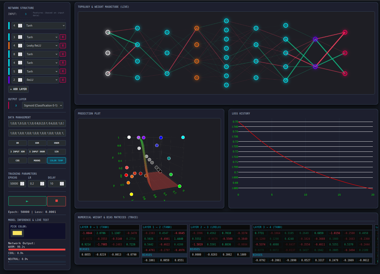
If you want to visualize how the training process happens, I have made a visualizer to tinker around. Please visit visualizer.

Matrix Multiplication Revisited: The Need for Speed

In our initial exploration of Linear Regression, we implemented a straightforward matrix multiplication. It was a literal translation of the mathematical definition—a triple-nested loop that worked perfectly for small datasets.

However, as we move toward Neural Networks, the scale changes. A single training session for a deep network requires performing hundreds to thousands of matrix multiplications per epoch. Although, we are not chasing peak performance in this guide, at this scale, the difference between “mathematically correct” and “machine-optimized” is the difference between training a model in minutes versus hours.

The Bottleneck: Why Naive is Slow

In standard textbooks, we learn the ijk order: iterate over rows of $A$ (the i loop), then columns of $B$ (the j loop), then sum the products (the k loop).

for i in 0..a_rows {
    for j in 0..b_cols {
        for k in 0..a_cols {
            result_data[i * b_cols + j] +=
                self.data[i * a_cols + k] * other.data[k * b_cols + j];
        }
    }
}

This implementation suffers from a classic hardware performance trap: Cache Locality.

The Problem: Jumping Across the Flat Buffer

In Rust, our Tensor data is a Vec<f32>, which is a Flat Buffer. Even though we think of a matrix as a square, the computer sees it as a single line.

Let’s look at a matrix :

\[B\ =\ \begin{bmatrix} \color{cyan}{1} & \color{magenta}{2} & 3 \\\ \color{cyan}{4} & \color{magenta}{5} & 6 \end{bmatrix}\]

In memory (RAM), it is laid out like this:

\[\text{RAM Index: }\underbrace{[\color{cyan}{1}\ \color{magenta}{2}\ \color{white}{3}]}_{Row 0}\ \underbrace{[\color{cyan}{4}\ \color{magenta}{5}\ \color{white}{6}]}_{Row 1}\]

Even though we visualize a matrix as a square, the computer sees it as a Flat Buffer in memory. When we jump across different rows of matrix $B$ to calculate a single element, the CPU is forced to constantly fetch new data from the slow RAM into its fast Cache.

The Evolution: From Loops to Iterators

To fix this, we need to rethink how we traverse memory. By rearranging our loops to an ikj order and utilizing Rust’s idiomatic iterators, we can transform our matmul function into a high-performance engine.

This loop order matters more than the math itself.

//src/tensor.rs
pub fn matmul(&self, other: &Tensor) -> Result<Tensor, TensorError> {
    // Shape Check and Normalization, same as naive multiplication

    // The core optimization: IKJ order with Iterators
    for (i, a_row) in self.data.chunks_exact(a_cols).enumerate() {
        let out_row_start = i * b_cols;
        let out_row = &mut data[out_row_start..out_row_start + b_cols];

        for (k, &aik) in a_row.iter().enumerate() {
            if aik == 0.0 {
                continue;
            } // Skip zeros for a small speed boost

            let b_row_start = k * b_cols;
            let b_row = &other.data[b_row_start..b_row_start + b_cols];

            // This zip() is the key to SIMD and removing bounds checks
            for (out_val, &b_val) in out_row.iter_mut().zip(b_row.iter()) {
                *out_val += aik * b_val;
            }
        }
    }

    // Forming return tensor
}

Up to this point, nothing mathematically has changed. We are still computing the same dot products, summing the same values, and producing the same result matrix.

To review the full mathematical derivation and how the optimized method performs the calculation, check Appendix B

Why This Is Faster

1. Cache-Friendly Access (IKJ Order): By moving the k loop outside the j loop, we process Matrix row by row. Since is stored in Row-Major order in our flat buffer, the CPU reads contiguous blocks of memory. This allows the hardware to pre-fetch data efficiently, minimizing “cache misses.”
2. Eliminating Bounds Checks: In the naive version, every access like data[i * b_cols + j] requires the Rust runtime to verify the index is within bounds. By using .chunks_exact() and .zip(), we provide the compiler with proof of the slice lengths, allowing it to strip away those expensive safety checks.
3. Enabling SIMD: The zip() iterator over contiguous slices is a signal to the LLVM compiler. It can often “auto-vectorize” this loop, using SIMD (Single Instruction, Multiple Data) instructions to multiply 4 or 8 floating-point numbers in a single CPU cycle.
4. Zero-Skipping: In neural networks, many weights or activations (especially after a ReLU layer) are exactly zero. A simple if aik == 0.0 { continue; } allows us to skip an entire row-worth of multiplications and additions.

Benchmark: The Reality of Optimization

When we compare our naive implementation against the optimized version, the performance gap widens drastically as the scale increases:

Matrix Size	Naive Time	Optimized Time	Speedup
2 x 2	742 ns	741 ns	1.00x
16 x 16	9.648 µs	1.533 µs	6.29x
128 x 128	7.859 ms	350.634 µs	22.42x

While absolute timings vary by hardware, the relative speedup remains consistent. You can run the demo to see these benchmarks on your own machine.

Checkpoint

If you only remember one thing from this section, remember this: changing loop order does not change math—but it completely changes performance. This is the difference between knowing linear algebra and thinking like a systems programmer.

Neural Network

In the previous chapters, we saw how a machine “learns” the building blocks of a linear equation. By adjusting $m$ (slope) and $c$ (intercept), we could fit a straight line to our data. This technique is incredibly powerful for simple predictions, but the real world is rarely a straight line.

The Limitation of Linearity

Consider the image below. It’s a monochrome spiral—a classic example of a pattern that no single straight line can ever describe, no matter how much we “tweak” the weights:

assets/spiral_50.pbm

To reconstruct a pattern like this, we need to support non-linearity in our library. In a linear model, even if we stack multiple layers, we get a bigger linear function.

Let’s take an example with two linear equations:

\[g(x) = n \cdot x + d\] \[f(x) = m \cdot g(x) + c \implies f(x) = m \cdot (n \cdot x + d) + c \implies f(x) = m \cdot n \cdot x + m \cdot d + c\]

Here $m$, $n$, $c$ and $d$ are all $constants$, so the final function again becomes - $f(x) = mx + c$, just with different values of $m$ and $c$.

Activation Function

To achieve non-linearity, we’ll wrap our existing linear function inside a non-linear Activation Function as follows:

\[f(x) = activation(linear(x)) = activation(X \cdot W + B)\]

Let’s take a real example:

\[g(x) = max(0, x)\] \[f(x) = 3 \cdot x + 5\] \[h(x) = g(f(x)) = max(0, (3 \cdot x + 5))\]

Let’s now plot this function for 10 points and see:

{
  "title": "Rectified Linear Unit",
  "traces": [
    {
      "type": "line",
      "x": [-5, -4, -3, -2, -1,  0,  1,  2,  3,  4],
      "y": [ 0,  0,  0,  0,  2,  5,  8, 11, 14, 17],
      "name": "ReLU"
    }
  ]
}

As you can see, with just one activation function, we can bend a straight line.

Implementing Activation

Let’s bring this mathematical part into code. We’ll create an activation.rs first. We’ll follow the same structure we followed in Linear Layer earlier:

use crate::tensor::Tensor;
use crate::tensor::TensorError;

pub enum ActivationType {
    ReLU,
}
pub struct Activation {
    input: Tensor,
    t: ActivationType,
}

impl Activation {
    pub fn new(t: ActivationType) -> Self {
        Activation {
            input: Tensor::empty(),
            t,
        }
    }
    pub fn forward(&mut self, input: &Tensor) -> Result<Tensor, TensorError> {
        self.input = Tensor::new(input.data().to_vec(), input.shape().to_vec())?;

        match self.t {
            ActivationType::ReLU => input.relu(),
        }
    }
}

Our tensor does not have relu defined yet. Let’s implement that inside our Tensor:

pub fn relu(&self) -> Result<Tensor, TensorError> {
    self._element_wise_op_single(|a| if a > 0.0 { a } else { 0.0 })
}

Now, let’ write the driver code:

fn main() -> Result<(), TensorError> {
    let mut rng = SimpleRng { state: 73 };

    let mut linear_layer = Linear::new(2, 1, &mut rng);
    let mut activation_layer = Activation::new(ActivationType::ReLU);

    let input = Tensor::new(
        vec![
            -2.0, 1.0_f32, -1.0, 1.0_f32, 0.0, 1.0_f32, 1.0, 1.0_f32, 2.0, 1.0_f32,
        ],
        vec![5, 2],
    )?;

    println!("Input:");
    println!("{}", input);

    let linear_output = linear_layer.forward(&input)?;

    println!("Linear Layer Output:");
    println!("{}", linear_output);

    let activation_output = activation_layer.forward(&linear_output)?;

    println!("Activation Layer Output");
    println!("{}", activation_output);

    Ok(())
}

Here is the output:

$ target/release/build-your-own-nn 
Input:
  | -2.0000,   1.0000|
  | -1.0000,   1.0000|
  |  0.0000,   1.0000|
  |  1.0000,   1.0000|
  |  2.0000,   1.0000|

Linear Layer Output:
  | -0.5247|
  | -0.1546|
  |  0.2155|
  |  0.5855|
  |  0.9556|

Activation Layer Output
  |  0.0000|
  |  0.0000|
  |  0.2155|
  |  0.5855|
  |  0.9556|

Please note that the negative values in the linear layer output has been transformed to 0 in the activation layer output. And if we plot the output, we’ll see some non-linearity in it.

{
  "title": "Forward Pass",
  "traces": [
    {
      "type": "line",
      "x": [-2, -1, 0, 1, 2],
      "y": [ 0, 0, 0.2155, 0.5855, 0.9566],
      "name": "ReLU"
    }
  ]
}

Our implementation already started forming a network. This simple network with one linear layer and one activation layer is known as Single Layer Perceptron in the world of Machine Learning. However, it is not complete yet. To achieve the status fully, we need to implement the mathematics of Backward Pass.

Backward Pass

The backward pass is not different from what we’ve already seen in linear regression. The same mathematics apply here too. Only difference is that, instead of propagating the loss to only one layer, we propagate it back to every layer. For now, we only have one layer of merged linear layer and activation layer. So our backward pass will look like this:

\[\text{Input} \leftarrow{} \text{Linear Layer} \leftarrow{} Output\]

Conceptually the network as a whole will look like this:

\[\begin{array}{ccccccc} X & \xrightarrow{W} & Z & \xrightarrow{\text{ReLU}} & A & \rightarrow & \text{Loss}(A, Y) \\ & & & & & & \downarrow \\ \frac{\partial L}{\partial X} & \xleftarrow{\text{Linear Grad}} & \frac{\partial L}{\partial Z} & \xleftarrow{\text{ReLU Grad}} & \frac{\partial L}{\partial A} & \leftarrow & \nabla \text{Loss} \end{array}\]

Implementing Single Layer Perceptron

Let’s complete the full flow.

We’ll start by writing the derivative of ReLU. By looking at the mathematical expression and the plot of ReLU function, it is clear that:

\[\frac{d}{dx}\text{ReLU}(x) = \begin{cases} 1 & \text{if } x > 0 \\ 0 & \text{otherwise} \end{cases}\]

We’ll add this function in our tensor:

pub fn relu_prime(&self) -> Result<Tensor, TensorError> {
    self._element_wise_op_single(|a| if a > 0.0 { 1.0 } else { 0.0 })
}

Now, we’ll add the backward method in our activation layer implementation:

pub fn backward(&self, output_error: &Tensor) -> Result<Tensor, TensorError> {
    match self.t {
        ActivationType::ReLU => {
            let mask = self.input.relu_prime()?;
            output_error.mul(&mask)
        }
    }
}

Finally, we would add the driver code:

fn main() -> Result<(), TensorError> {
    let mut rng = SimpleRng { state: 73 };

    let mut linear_layer = Linear::new(2, 1, &mut rng);
    let mut activation_layer = Activation::new(ActivationType::ReLU);

    let input = Tensor::new(vec![0.0, 0.0, 0.0, 1.0, 1.0, 0.0, 1.0, 1.0], vec![4, 2])?;
    let actual = Tensor::new(vec![0.0, 1.0, 1.0, 1.0], vec![4, 1])?;

    let learning_rate = 0.01;

    println!("Input:");
    println!("{}", input);

    println!("Actual Input");
    println!("{}", actual);

    for _ in 0..5000 {
        let linear_output = linear_layer.forward(&input)?;
        let activation_output = activation_layer.forward(&linear_output)?;

        let grad = mse_loss_gradient(&activation_output, &actual)?;

        let activation_grad = activation_layer.backward(&grad)?;

        let _ = linear_layer.backward(&activation_grad, learning_rate);
    }

    let model_output = linear_layer.forward(&input)?;
    let model_output = activation_layer.forward(&model_output)?;

    println!("Model Output after training");
    println!("{}", model_output);

    Ok(())
}

We are using the OR gate expression to approximate by our network and here is the network output:

$ target/release/build-your-own-nn 
Input:
  |  0.0000,   0.0000|
  |  0.0000,   1.0000|
  |  1.0000,   0.0000|
  |  1.0000,   1.0000|

Actual Output
  |  0.0000|
  |  1.0000|
  |  1.0000|
  |  1.0000|

Model Output after training
  |  0.0000|
  |  0.6667|
  |  0.6667|
  |  1.3333|

The network is separating the data. However, it can do better, if we add a few more loss and activations.

Sigmoid Activation & BCE Loss

MSE is great for Regression problems but Binary Cross Entropy suits better for binary classification problems, where the output is either $0$ or $1$. Similarly, for activation functions ReLU is used widely in many applications but we will also encounter a few more while working with neural networks. In particular Sigmoid is used widely for binary classification problems.

Let’s look at the definitions of these functions, their derivatives and add them in our application.

Sigmoid

Sigmoid is defined mathematically as:

\[\sigma(x) = \frac{1}{1 + e^{-x}}\]

This is the shape of the function:

{
  "title": "Sigmoid",
  "traces": [
    {
      "type": "line",
      "x": [-6.0, -5.0       , -4.47368421, -3.94736842, -3.42105263, -2.89473684,
            -2.36842105, -1.84210526, -1.31578947, -0.78947368, -0.26315789,
            0.26315789,  0.78947368,  1.31578947,  1.84210526,  2.36842105,
            2.89473684,  3.42105263,  3.94736842,  4.47368421,  5.0, 6],
      "y": [0.00247, 0.00669285, 0.01127661, 0.0189398 , 0.03164396, 0.05241435,
            0.08561266, 0.1368025 , 0.21151967, 0.31228169, 0.43458759,
            0.56541241, 0.68771831, 0.78848033, 0.8631975 , 0.91438734,
            0.94758565, 0.96835604, 0.9810602 , 0.98872339, 0.99330715, 0.9975273768433653],
      "name": ""
    }
  ]
}

Notice that this function squeezes any value between $0$ and $1$. This feature acts as a probability map and is useful for classification problems.

Its derivative is defined as:

\[\frac{d}{dx}\sigma(x) = \sigma(x) \cdot (1 - \sigma(x))\]

To implement both these functions we’ll need exp method in our tensor. Let’s add that in tensor.

pub fn exp(&self) -> Result<Tensor, TensorError> {
    self._element_wise_op_single(|a| f32::exp(a))
}

We have to extend our tensor to give us a tensor filled with all $1$. We could do it with by simply creating a vec![1; size] too but one is a handy method.

pub fn one(shape: Vec<usize>) -> Result<Tensor, TensorError> {
    if shape.len() == 0 || shape.len() > 2 {
        return Err(TensorError::InvalidRank);
    }
    
    let data = vec![1.0; shape.iter().product()];
    
    Ok(Tensor { data, shape })
}

Let’s create the implementation in activation as well:

impl Activation {
    pub fn new(t: ActivationType) -> Self {
        Activation {
            input: Tensor::empty(),
            t,
        }
    }
    pub fn forward(&mut self, input: &Tensor) -> Result<Tensor, TensorError> {
        self.input = Tensor::new(input.data().to_vec(), input.shape().to_vec())?;

        match self.t {
            ActivationType::ReLU => input.relu(),
            ActivationType::Sigmoid => {
                let neg_x = input.scale(&-1.0)?;
                let denominator = Tensor::one(input.shape().to_vec())?.add(&neg_x.exp()?)?;

                Tensor::one(input.shape().to_vec())?.div(&denominator)
            }
        }
    }

    pub fn backward(&self, output_error: &Tensor) -> Result<Tensor, TensorError> {
        match self.t {
            ActivationType::ReLU => {
                let mask = self.input.relu_prime()?;
                output_error.mul(&mask)
            }

            ActivationType::Sigmoid => {
                let neg_input = self.input.scale(&-1.0)?;
                let denominator =
                    Tensor::one(self.input.shape().to_vec())?.add(&neg_input.exp()?)?;
                let a = Tensor::one(self.input.shape().to_vec())?.div(&denominator)?;

                let one = Tensor::one(a.shape().to_vec())?;
                let sigmoid_prime = a.mul(&one.sub(&a)?)?;

                output_error.mul(&sigmoid_prime)
            }
        }
    }
}

Finally, we’ll rewrite the driver code.

fn main() -> Result<(), TensorError> {
    let mut rng = SimpleRng { state: 73 };

    let mut linear_layer = Linear::new(3, 1, &mut rng);
    let mut activation_layer = Activation::new(ActivationType::Sigmoid);

    let input = Tensor::new(
        vec![
            0.0, 0.0, 1.0_f32, 0.0, 1.0, 1.0_f32, 1.0, 0.0, 1.0_f32, 1.0, 1.0, 1.0_f32,
        ],
        vec![4, 3],
    )?;
    let actual = Tensor::new(vec![0.0, 1.0, 1.0, 1.0], vec![4, 1])?;

    let learning_rate = 0.1;

    println!("Input:");
    println!("{}", input);

    println!("Actual Output");
    println!("{}", actual);

    for _ in 0..5000 {
        let linear_output = linear_layer.forward(&input)?;
        let activation_output = activation_layer.forward(&linear_output)?;

        let grad = bce_sigmoid_delta(&activation_output, &actual)?;

        let activation_grad = activation_layer.backward(&grad)?;

        let _ = linear_layer.backward(&activation_grad, learning_rate);
    }

    let model_output = linear_layer.forward(&input)?;
    let model_output = activation_layer.forward(&model_output)?;

    println!("Model Output after training");
    println!("{}", model_output);

    Ok(())
}

We can clearly see the network has learnt the pattern better than our old architecture with MSE:

$ target/release/build-your-own-nn 
Input:
  |  0.0000,   0.0000,   1.0000|
  |  0.0000,   1.0000,   1.0000|
  |  1.0000,   0.0000,   1.0000|
  |  1.0000,   1.0000,   1.0000|

Actual Output
  |  0.0000|
  |  1.0000|
  |  1.0000|
  |  1.0000|

Model Output after training
  |  0.1781|
  |  0.8926|
  |  0.8928|
  |  0.9969|

Sigmoid BCE Shortcut

We are still using the MSE to calculate the loss. However, if we pair Sigmoid and BCE, we get a shortcut to use without all the expensive operations. In the shortcut step, we don’t calculate the loss and the gradient separately, we fuse them together to get: $grad=(a-y)$.

We add the shortcut in the loss module:

pub fn bce_sigmoid_delta(predicted: &Tensor, actual: &Tensor) -> Result<Tensor, TensorError> {
    if predicted.shape() != actual.shape() {
        return Err(TensorError::ShapeMismatch);
    }

    let n = predicted.shape().iter().product::<usize>() as f32;
    
    predicted.sub(actual)?.scale(&(1.0 / n))
}

Then change our training loop:

for _ in 0..5000 {
    let linear_output = linear_layer.forward(&input)?;
    let activation_output = activation_layer.forward(&linear_output)?;

    let delta = bce_sigmoid_delta(&activation_output, &actual)?;

    let _ = linear_layer.backward(&delta, learning_rate);
}

Limitation of Single Layer Perceptron

We have successfully stacked layers of calculations and we have seen how we can use this to classify things into yes/no category. However, this architecture cannot generalize to any functions. This only works for linearly separable data or data which has a clear separating lines into two categories. Like OR, AND, NAND, NOR etc. logic. Let’s see the line of separation in these cases.

{
  "title": "OR Gate Decision Boundary",
  "layout": {
    "xaxis": { "title": "Input X1", "range": [-0.5, 1.5] },
    "yaxis": { "title": "Input X2", "range": [-0.5, 1.5] },
    "showlegend": false
  },
  "traces": [
    {
      "type": "contour",
      "x": [-0.5, 0, 0.5, 1.0, 1.5],
      "y": [-0.5, 0, 0.5, 1.0, 1.5],
      "z": [
        [0.26, 0.37, 0.50, 0.62, 0.73],
        [0.37, 0.50, 0.62, 0.73, 0.81],
        [0.50, 0.62, 0.73, 0.81, 0.88],
        [0.62, 0.73, 0.81, 0.88, 0.92],
        [0.73, 0.81, 0.88, 0.92, 0.95]
      ],
      "colorscale": [
                        [0, "#964440"],
                        [1, "#368d3e"]
                    ],
      "reversescale": false,
      "showscale": true,
      "contours": {
        "coloring": "heatmap",
        "showlines": true,
        "start": 0.5,
        "end": 0.5,
        "size": 0
      }
    },
    {
      "type": "scatter",
      "x": [0, 0, 1, 1],
      "y": [0, 1, 0, 1],
      "mode": "markers",
      "marker": {
        "size": 18,
        "color": [0, 1, 1, 1],
        "colorscale": [
             [0, "#e73027"],
             [1, "#1bd82e"]
        ],
        "reversescale": false,
        "line": { "width": 3, "color": "white" },
        "symbol": "circle"
      },
      "name": "Actual Data"
    }
  ]
}

In this, the black line is the decision boundary.

Let’s check out the similar for XOR gate:

{
  "title": "XOR Gate Decision Boundary (Non-Linear)",
  "layout": {
    "xaxis": { "title": "Input X1", "range": [-0.5, 1.5] },
    "yaxis": { "title": "Input X2", "range": [-0.5, 1.5] },
    "showlegend": false
  },
  "traces": [
    {
      "type": "contour",
      "x": [-0.5, 0, 0.5, 1.0, 1.5],
      "y": [-0.5, 0, 0.5, 1.0, 1.5],
      "z": [
        [0.10, 0.30, 0.45, 0.30, 0.10],
        [0.30, 0.10, 0.80, 0.95, 0.60],
        [0.45, 0.80, 0.50, 0.80, 0.45],
        [0.30, 0.95, 0.80, 0.10, 0.30],
        [0.10, 0.60, 0.45, 0.30, 0.10]
      ],
      "colorscale": [
                        [0, "#964440"],
                        [1, "#368d3e"]
                    ],
      "reversescale": true,
      "showscale": true,
      "contours": {
        "coloring": "heatmap",
        "showlines": true,
        "start": 0.5,
        "end": 0.5,
        "size": 0
      }
    },
    {
      "type": "scatter",
      "x": [0, 1, 0, 1],
      "y": [0, 1, 1, 0],
      "mode": "markers",
      "marker": {
        "size": 18,
        "color": [0, 0, 1, 1],
        "colorscale": [
             [0, "#e73027"],
             [1, "#1bd82e"]
        ],
        "reversescale": true,
        "line": { "width": 3, "color": "white" },
        "symbol": "circle"
      },
      "name": "Actual Data"
    }
  ]
}

Here you’ll see XOR gate doesn’t have a linear decision boundary. A single layer perceptron can’t approximate this.

Let’s try it with our network. We’ll simply change the last output of OR ($1$) to output of XOR ($0$).

let actual = Tensor::new(vec![0.0, 1.0, 1.0, 0.0], vec![4, 1])?;

Output:

$ target/release/build-your-own-nn 
Input:
  |  0.0000,   0.0000,   1.0000|
  |  0.0000,   1.0000,   1.0000|
  |  1.0000,   0.0000,   1.0000|
  |  1.0000,   1.0000,   1.0000|

Actual Output
  |  0.0000|
  |  1.0000|
  |  1.0000|
  |  0.0000|

Model Output after training
  |  0.5000|
  |  0.5000|
  |  0.5000|
  |  0.5000|

The network squashed every output to the same number. Even if we change our activation and loss functions, the network won’t be able to approximate the function.

Does it mean, we are stuck here?

Of course not. We solve the problem with Multi Layer Perceptron.

Multi Layer Perceptron

We have experienced, a single layer perceptron can’t generalize any approximation. This is where we start leaning on our creativity to solve the problem of generalization. We use Single Layer Perceptron as a unit rather than final product.

We stack a combination of Single Layer Perceptrons and we can approximate any continuous function — a principle known as Universal Approximation Theorem.

According to wikipedia —

the universal approximation theorems (UATs) state that neural networks with a certain structure can, in principle, approximate any continuous function to any desired degree of accuracy.

We’ll now see it in action.

Our linear equation definition is:

\[f(x) = 3 \cdot x + 5\]

The ReLU defintion is:

\[g(x) = max(0, x) %\]

A single layer of combined function is:

\[act(x) = g(f(x)) = max(0, (3 \cdot x + 5))\]

Finally two layers of stacking gives us:

\[h(x) = g(f(g(f(x)))) = max(0, 3 \cdot (max(0, 3 \cdot x + 5)) + 5)\]

{
  "title": "Rectified Linear Unit",
  "traces": [
    {
      "type": "line",
      "x": [-5, -4, -3, -2, -1,  0,  1,  2,  3,  4],
      "y": [ 0,  0,  0,  0,  2,  5,  8, 11, 14, 17],
      "name": "Single Layer"
    },
    {
      "type": "line",
      "x": [-5, -4, -3, -2, -1,  0,  1,  2,  3,  4],
      "y": [ 5,  5,  5,  5, 11, 20, 29, 38, 47, 56],
      "name": "2 Layers"
    }
  ]
}

With a single layer of ReLU, we bring a bend in the straight line produced by the linear equation. As we move on stacking layers, the bend in the activation function becomes more complex, allowing the model to fit non-linear data.

We’ll now see what happens if we mix two different valued $m$ and $c$ and add them together.

\[y_{1}(x) = 3x+2\] \[y_{2}(x) = -3x+4\] \[f(x) = max(0,x)\] \[y = f(y_{1}(x)) - f(y_{2}(x)) = max(0, 3x + 2) + max(0, -3x + 4)\]

{
  "title": "Rectified Linear Unit",
  "traces": [
    {
      "type": "line",
      "x": [-5, -4, -3, -2, -1,  0,  1,  2,  3,  4],
      "y": [ 19, 16, 13, 10,  7,  6,  6,  8, 11, 14],
      "name": "2 Different Units Added"
    }
  ]
}

This combination is now enough to not only bend the straight line in one direction but in all directions. If we use these two stacking mechanisms together we can approximate any complex function. We control the bend using different values of $m$ and $c$.

We have already used $calculus$ to derive the nearest values of the slope and bias by calculating the loss from actual data. Here also we do the same. We derive the correct slopes and biases which shapes any function. Hence, Deep Learning is Reverse Engineering on steroids.

TIP

It is a bit more involved. I recommend visiting Desmos and plotting a few of the techniques discussed in this section by plotting the stacked functions yourselves to get hands on experience.

Implementation

Once we have strengthened our mental model, we are ready to write some code. We actually have all the pieces ready. We just stack these pieces together and can start writing the driver code. We’ll start with where left in the last section and approximated the XOR gate and stack one more layer to it:

pub fn xor_neural_network(rng: &mut dyn Rng) -> Result<(), TensorError> {

    let mut input_layer = Linear::new(3, 4, rng);
    let mut activation_layer = Activation::new(ActivationType::ReLU);

    // These two lines creates the new layer
    let mut hidden_layer = Linear::new(4, 1, rng);
    let mut hidden_activation = Activation::new(ActivationType::Sigmoid);

    let input = Tensor::new(vec![0.0, 0.0, 1.0_f32, 0.0, 1.0, 1.0_f32, 1.0, 0.0, 1.0_f32, 1.0, 1.0, 1.0_f32], vec![4, 3])?;

    // Notice the change in the actual output
    let actual = Tensor::new(vec![0.0, 1.0, 1.0, 0.0], vec![4, 1])?;

    let learning_rate = 0.1;

    println!("Input:");
    println!("{}", input);

    println!("Actual Output");
    println!("{}", actual);

    for _ in 0..5_000 {
        let linear_output = input_layer.forward(&input)?;
        let activation_output = activation_layer.forward(&linear_output)?;

        // Following two lines are stacking the new layer on top of the existing
        let hidden_output = hidden_layer.forward(&activation_output)?;
        let hidden_activation_output = hidden_activation.forward(&hidden_output)?;

        let delta = bce_sigmoid_delta(&hidden_activation_output, &actual)?;

        // Loss is also passed in reverse direction from output to input
        let hidden_backward = hidden_layer.backward(&delta, learning_rate)?;
        let activation_backward = activation_layer.backward(&hidden_backward)?;

        let _ = input_layer.backward(&activation_backward, learning_rate);

    }

    let model_output = input_layer.forward(&input)?;
    let model_output = activation_layer.forward(&model_output)?;

    // During prediction also, the input should pass through the stacked layers.
    let model_output = hidden_layer.forward(&model_output)?;
    let model_output = hidden_activation.forward(&model_output)?;

    println!("Model Output after training");
    println!("{}", model_output);

    Ok(())
}

The above function results:

Input:
  |  0.0000,   0.0000,   1.0000|
  |  0.0000,   1.0000,   1.0000|
  |  1.0000,   0.0000,   1.0000|
  |  1.0000,   1.0000,   1.0000|

Actual Output
  |  0.0000|
  |  1.0000|
  |  1.0000|
  |  0.0000|

Model Output after training
  |  0.0024|
  |  0.5000|
  |  0.9988|
  |  0.0019|

You may get a slightly different result but you can see, our new stacked network is doing a better approximation. Yet it is not still giving a satisfactory approximation. This is the right place we talk about another significant approach in Machine Learning, known as ‘Hyperparameter tuning’.

Hyperparameter Tuning

We now have the network ready, we have the layers working for us, math is being implemented as expected. Yet we don’t see a satisfactory answer. The network correctly maked 3 out of 4 answers but it could not approximate one value, the second number in the output $0.5000$. Looks like, it is stuck on the boundary where it is not sure if it should go to $0$ or $1$.

This is exactly where, we need to do a few set of experiments to determine the best model. The best model highly depends on the dataset being used for training. Hence, there is no specific rule for setting these parameters. We just experiment. These experiments can be manual or can be done through automation but the idea remains the same; tinker around the settings in search of the best suit.

We already are using two hyperparameters from our first model of linear regression. We started with a hunch and for all the experiments we have done, that hunch worked for us smoothly. However, as the complexity grew that initial hunch seems to be not working any more.

Here are the two hyperparameters we are using from the begining - learning rate and epoch.

From this section onwards, we’ll use two more - number of layers and number of nodes per layer.

As you have already seen, to stack a new layer to the network, we have to make changes in code and we have to keep track of the order of the layers in both the passes.

Let’s refactor the code. We’ll perform these actions:

• The forward and backward methods will be required for each layer. We’ll unify these two methods in a trait
• we’ll create a new module neural_network.rs which will hold the layers
• We’ll make a forward method which we’ll use for both forward pass and predictions
• We’ll create a fit method for training
• We’ll expose APIs to add layers to the neural network
• We’ll write a builder struct to build the network for cleaner access
• We’ll write a driver method which uses the network module and the builder module

Here is the code for neural network and its builder module:

use crate::Layer;
use crate::tensor::{Tensor, TensorError};

/// Type alias for the loss gradient function pointer
type LossGradFn = fn(&Tensor, &Tensor) -> Result<Tensor, TensorError>;

pub struct Network {
    layers: Vec<Box<dyn Layer>>,
    loss_grad_fn: LossGradFn,
}

impl Network {
    /// Passes the input through all layers sequentially
    pub fn forward(&mut self, input: Tensor) -> Result<Tensor, TensorError> {
        if self.layers.is_empty() {
            return Ok(input);
        }

        let mut current_output = input;

        for layer in &mut self.layers {
            // Each layer processes the output of the previous layer
            current_output = layer.forward(&current_output)?;
        }

        Ok(current_output)
    }

    /// The training loop: Forward, Loss Gradient, and Backpropagation
    pub fn fit(
        &mut self,
        x_train: &Tensor,
        y_train: &Tensor,
        epochs: usize,
        learning_rate: f32,
    ) -> Result<(), TensorError> {
        for epoch in 0..epochs {
            // Following is the forward pass
            let input = Tensor::new(x_train.data().to_vec(), x_train.shape().to_vec())?;
            let output = self.forward(input)?;

            // Loss gradient
            let mut gradient = (self.loss_grad_fn)(&output, y_train)?;

            // Passing the gradient backward from output to input
            for layer in self.layers.iter_mut().rev() {
                gradient = layer.backward(&gradient, learning_rate)?;
            }
        }
        Ok(())
    }
}

/// Builder pattern for cleaner Network initialization
pub struct NetworkBuilder {
    layers: Vec<Box<dyn Layer>>,
    loss_grad: Option<LossGradFn>,
}

impl NetworkBuilder {
    pub fn new() -> Self {
        Self {
            layers: Vec::new(),
            loss_grad: None,
        }
    }

    /// Adds a layer to the network stack
    pub fn add_layer(mut self, layer: Box<dyn Layer>) -> Self {
        self.layers.push(layer);
        self
    }

    /// Injects the loss gradient function from loss.rs
    pub fn loss_gradient(mut self, f: LossGradFn) -> Self {
        self.loss_grad = Some(f);
        self
    }

    pub fn build(self) -> Result<Network, String> {
        let loss_grad_fn = self.loss_grad.ok_or("Loss gradient function is required")?;

        Ok(Network {
            layers: self.layers,
            loss_grad_fn,
        })
    }
}

The refactored driver code now got simplified. If we want to change any hyperparameter and test, we can simply make few changes and the rest will be taken care automatically.

use crate::{
    Rng,
    activation::{Activation, ActivationType},
    linear::Linear,
    loss::bce_sigmoid_delta,
    neural_network::NetworkBuilder,
    tensor::{Tensor, TensorError},
};

pub fn xor_neural_network(rng: &mut dyn Rng) -> Result<(), TensorError> {
    let mut nn = NetworkBuilder::new()
        .add_layer(Box::new(Linear::new(3, 12, rng)))
        .add_layer(Box::new(Activation::new(ActivationType::ReLU)))
        .add_layer(Box::new(Linear::new(12, 1, rng)))
        .add_layer(Box::new(Activation::new(ActivationType::Sigmoid)))
        .loss_gradient(bce_sigmoid_delta)
        .build()
        .expect("Error building network");

    let input = Tensor::new(
        vec![0.0, 0.0, 1.0, 0.0, 1.0, 1.0, 1.0, 0.0, 1.0, 1.0, 1.0, 1.0],
        vec![4, 3],
    )?;

    let actual = Tensor::new(vec![0.0, 1.0, 1.0, 0.0], vec![4, 1])?;

    println!("Input:\n{}", input);
    println!("Actual Output:\n{}", actual);

    println!("Training...");
    nn.fit(&input, &actual, 20_000, 0.01)?;

    let model_output = nn.forward(input)?;

    println!("Model Output after training:\n{}", model_output);

    Ok(())
}

We have now simplified the whole training process. With just a few lines of code, we can now train the network with data.

Two Moons Experiment

To verify that the system can learn genuinely non-linear structure, we evaluate it on the two moons dataset. This dataset cannot be separated by a linear model and therefore serves as a useful diagnostic rather than a benchmark.

With a small increase in network capacity, the model learns a curved decision boundary directly from the data:

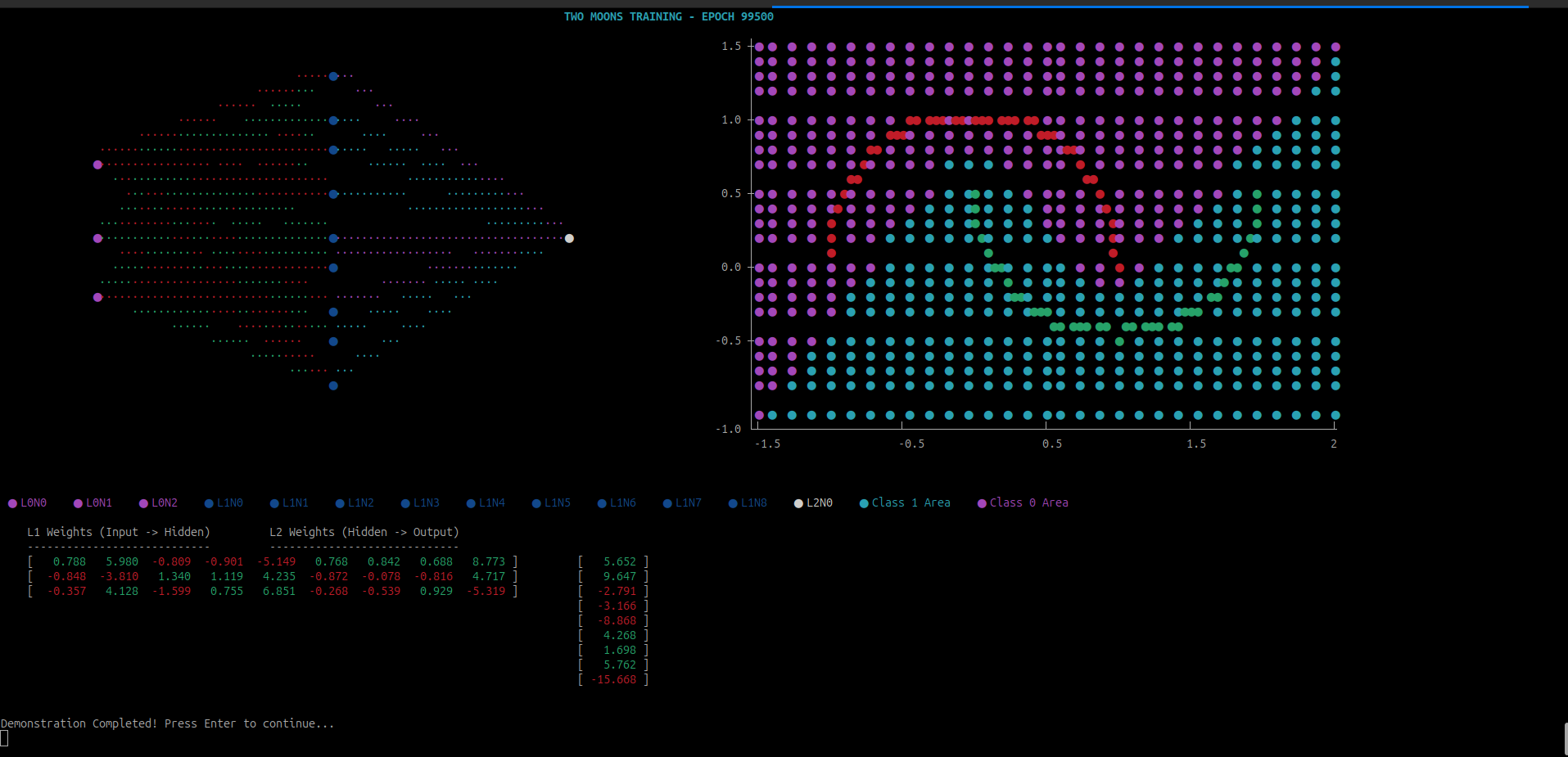
The plotting and drawing machinery used to generate this visualization is intentionally kept separate from the learning system. Details of the visualization pipeline are described in Appendix C

Checkpoint

That covers the fundamentals of Deep Learning. This is the foundation. From here, you can begin your journey with complex architectures like:

1. N-Gram Generators
2. Convolutional Neural Networks (CNNs)
3. Recurrent Neural Networks (RNNs)
4. Image Recognition
5. LSTM Networks
6. Transformers

No matter which path you take next, the fundamentals remain the same. Even a trillion-parameter Transformer model with emergent intelligence follows these basics.

To see these basics in action, we will now move from theoretical models to a practical application. In the next chapter, we will build a neural network that learns to perform Image Reconstruction, transforming a low-resolution 25×25 spiral into a sharp, high-fidelity 200×200 image.

TIP

I have built a Neural Network Visualizer for you to tinker around. If you want to quickly verify how Neural Network works under the hood, head over to the hosted Neural Network Visualizer.

Image Reconstruction: From Data to Geometry

This is our ultimatum. We built the machinery to perform this task specifically. This will give us the exact visual proof and justify all the pain we endured while tracing the mathematics.

We’ll take a $50 \times 50$ PBM and reconstruct it on $200 \times 200$ canvas.

The Portable BitMap (PBM)

Throughout this guide, we have maintained a No Third Party stance, this chapter will not be an exception. To keep up with the theme, we’ll use the Portable BitMap (PBM) format.

PBM is the simplest way of storing an image. It is a text based image format, which can be opened in a text editor.

For example, the following is a simple $5 \times 5$ checkerboard image:

P1
5 5
1 0 1 0 1
0 1 0 1 0
1 0 1 0 1
0 1 0 1 0
1 0 1 0 1

If you open a textbox, copy and paste the code above and save the file with .pbm extension, you can see your image viewer opening this as a very tiny checkerbox image.

PBM has the top lines dedicated to the description. The first line gives the magic number P1 and the second line describes the width and height. The following matrix describes the pixel values - $0$ means white pixel and $1$ means black pixel.

That’s all about PBM we need to know, for more details checkout this WIKIPEDIA Page.

The PBM Reader

PBM is a great choice for our use case, it directly gives us the input tensor without the need of any compression or decompression logic or any encoder/decoder.

With 20 lines of code, we can directly get the input matrix for our neural network:

pub fn read_pbm_for_nn(path: &str) -> (usize, usize, Vec<f32>, Vec<f32>) {
    let content = std::fs::read_to_string(path).expect("Read failed");
    let mut tokens = content.split_whitespace();

    assert_eq!(tokens.next().unwrap(), "P1");
    let w: usize = tokens.next().unwrap().parse().unwrap();
    let h: usize = tokens.next().unwrap().parse().unwrap();

    let mut x_coords = Vec::with_capacity(w * h * 2);
    let mut y_values = Vec::with_capacity(w * h);

    for i in 0..(w * h) {
        // Input: [Row, Col]
        x_coords.push((i / w) as f32); 
        x_coords.push((i % w) as f32);
        // Target: [Pixel]
        y_values.push(tokens.next().unwrap().parse().unwrap());
    }

    (w, h, x_coords, y_values)
}

In this code, we are taking the $(x, y)$ coordinates of the image as a single row. This is our training input or x_train. We are taking the pixel value at those coordinates. This corresponds to our target value or y_train. We can’t directly take the matrix as is. Otherwise, we’ll run into shape mismatch error while trying to reconstruct the same image in a different size.

The Tanh Activation Function

If you noticed this, relu has a problem. It has its own place in Machine Learning World, Image Reconstruction is not one of them. If you think about it, relu is essentially made of two straight lines. So, our network will try very hard to fit the curve of the spiral into thousands of straight lines. Theoritically we can draw any shape using straight lines but we live in a practical world where resources matter, especially when everything we built upto now is running on CPU. We can’t keep running the program forever. Patience plays a role too.

The another big reason to avoid relu in these contexts is it can kiil neurons by transforming any negative inputs to $0$ and so, it does not have a negative swing. Remember in our section on non-linearity discussion, we were manually choosing negative slopes to bring a bump in the stacked output of relu layers. While it is possible for a machine to assign a negative weight automatically but before it becomes creative with calculations and guesses many nodes might already be set to 0 by relu. Once this happens, there is no rescue and that neuron is dead forever.

To avoid these problems, we introduce a new activation function - Hyperbolic Tangent or in short tanh. This is how the function looks like:

{
    "title": "tanh",
    "traces":[
        {
            "type": "line",
            "x": [-5.0 , -4.47368421, -3.94736842, -3.42105263, -2.89473684,
                    -2.36842105, -1.84210526, -1.31578947, -0.78947368, -0.26315789,
                    0.26315789,  0.78947368,  1.31578947,  1.84210526,  2.36842105,
                    2.89473684,  3.42105263,  3.94736842,  4.47368421,  5.0],
            "y": [-0.9999092 , -0.99973988, -0.99925488, -0.99786657, -0.99389948,
                  -0.98261979, -0.95099682, -0.865733  , -0.65811078, -0.25724684,
                   0.25724684,  0.65811078,  0.865733  ,  0.95099682,  0.98261979,
                   0.99389948,  0.99786657,  0.99925488,  0.99973988,  0.9999092 ]
        }
    ]
}

This function looks like sigmoid function but instead of squeezing values between $0$ and $1$, this function squeezes them between $-1$ and $1$ and it has the similar curvature, sigmoid had. Thus this function can draw the curves in an image.

This is the mathematical definition of this function:

\[\tanh(x) = \frac{e^x - e^{-x}}{e^x + e^{-x}}\]

And its derivative:

\[\frac{d}{dx}\tanh(x) = 1 - \tanh^2(x)\]

We’ll add these in our activation module:

impl Layer for Activation {
    fn forward(&mut self, input: &Tensor) -> Result<Tensor, TensorError> {
        self.input = Tensor::new(input.data().to_vec(), input.shape().to_vec())?;

        match self.t {
            ActivationType::ReLU => input.relu(),
            ActivationType::Sigmoid => {
                let neg_x = input.scale(&-1.0)?;
                let denominator = Tensor::one(input.shape().to_vec())?.add(&neg_x.exp()?)?;

                Tensor::one(input.shape().to_vec())?.div(&denominator)
            }
            ActivationType::Tanh => {
                // Formula: (exp(x) - exp(-x)) / (exp(x) + exp(-x))
                let exp_x = input.exp()?;
                let exp_neg_x = input.scale(&-1.0)?.exp()?;

                let numerator = exp_x.sub(&exp_neg_x)?;
                let denominator = exp_x.add(&exp_neg_x)?;

                numerator.div(&denominator)
            }
        }
    }

    fn backward(&mut self, output_error: &Tensor, _: f32) -> Result<Tensor, TensorError> {
        match self.t {
            ActivationType::ReLU => {
                let mask = self.input.relu_prime()?;
                output_error.mul(&mask)
            }

            ActivationType::Sigmoid => {
                let neg_input = self.input.scale(&-1.0)?;
                let denominator =
                    Tensor::one(self.input.shape().to_vec())?.add(&neg_input.exp()?)?;
                let a = Tensor::one(self.input.shape().to_vec())?.div(&denominator)?;

                let one = Tensor::one(a.shape().to_vec())?;
                let sigmoid_prime = a.mul(&one.sub(&a)?)?;

                output_error.mul(&sigmoid_prime)
            }
            ActivationType::Tanh => {
                // Derivative: 1 - tanh^2(x)
                let exp_x = self.input.exp()?;
                let exp_neg_x = self.input.scale(&-1.0)?.exp()?;
                let tanh_x = exp_x.sub(&exp_neg_x)?.div(&exp_x.add(&exp_neg_x)?)?;

                let one = Tensor::one(tanh_x.shape().to_vec())?;
                let tanh_sq = tanh_x.mul(&tanh_x)?;
                let tanh_prime = one.sub(&tanh_sq)?;

                output_error.mul(&tanh_prime)
            }
        }
    }
}

The Feature Scaling

If we now go ahead and change our network to use $tanh$ instead, it will start working and will work for small images with may be upto 5 or 10 pixels but it will not work for higher resolution images. The reason behind that is the same $tanh$. Because at higher resolutions, we get values of x in high values. For example, our training image of $50$ pixels is also enough to push the tanh to the higher end of the function and the derivative becomes $0$, causing a Vanishing Gradient problem.

To overcome this issue, we use a technique called normalization.

let (w, h, x_data, y_data) = read_pbm_for_nn(source);

// Without Normalization, the gradient becomes zero. So, we make the data between 0 and 1
let normalized_x_train: Vec<f32> = x_data
    .chunks(2)
    .flat_map(|coord| vec![coord[0] / h as f32, coord[1] / w as f32])
    .collect();

There are many ways we do normalization, here we are simply dividing each pixel by the max value.

Network Architecture

This is where all the pieces finally come together and you can start experimenting with a complete network. I should be honest here as the author of this guide: I do not have a principled reason why this exact architecture works.

I arrived at it by trial and error. I have tried a few more that worked well too but this was by far the best architecture:

let hl = 64; // Hidden layer size
let mut nn = NetworkBuilder::new()
    .add_layer(Box::new(Linear::new(2, hl, rng)))
    .add_layer(Box::new(Activation::new(ActivationType::Tanh))) // For Image reconstruction tasks, Tanh is a better solution
    .add_layer(Box::new(Linear::new(hl, hl, rng)))
    .add_layer(Box::new(Activation::new(ActivationType::Tanh)))
    .add_layer(Box::new(Linear::new(hl, 2 * hl, rng))) // Expansion layer
    .add_layer(Box::new(Activation::new(ActivationType::Tanh)))
    .add_layer(Box::new(Linear::new(2 * hl, hl, rng))) // Contraction layer
    .add_layer(Box::new(Activation::new(ActivationType::Tanh)))
    .add_layer(Box::new(Linear::new(hl, hl / 2, rng)))
    .add_layer(Box::new(Activation::new(ActivationType::Tanh)))
    .add_layer(Box::new(Linear::new(hl / 2, 1, rng)))
    .add_layer(Box::new(Activation::new(ActivationType::Sigmoid))) // Final Sigmoid for pixel intensity
    .loss_gradient(bce_sigmoid_delta)
    .build()
    .map_err(|e| e.to_string())?;

This architecture looks like the following:

{
    "title": "Image Reconstructor Network Architecture",
    "removeGrid": true,
    "traces":[
        {
      "type": "scatter",
      "x": [0,0, 1,1,1,1,1,1,1,1, 2,2,2,2,2,2,2,2, 3,3,3,3,3,3,3,3,3,3,3,3,3,3,3,3, 4,4,4,4,4,4,4,4, 5,5,5,5,5,5,5,5, 6],
      "y": [0.5,-0.5, 3.5,2.5,1.5,0.5,-0.5,-1.5,-2.5,-3.5, 3.5,2.5,1.5,0.5,-0.5,-1.5,-2.5,-3.5, 7.5,6.5,5.5,4.5,3.5,2.5,1.5,0.5,-0.5,-1.5,-2.5,-3.5,-4.5,-5.5,-6.5,-7.5, 3.5,2.5,1.5,0.5,-0.5,-1.5,-2.5,-3.5, 3.5,2.5,1.5,0.5,-0.5,-1.5,-2.5,-3.5, 0],
      "hoverinfo": "none",
      "marker": {
        "size": 16,
        "color": [
          "white", "white", 
          "cyan", "cyan", "cyan", "cyan","cyan","cyan","cyan","cyan",
          "cyan", "cyan", "cyan", "cyan","cyan","cyan","cyan","cyan",
          "cyan", "cyan", "cyan", "cyan", "cyan", "cyan","cyan","cyan",
          "cyan", "cyan", "cyan", "cyan","cyan","cyan","cyan","cyan",
          "cyan", "cyan", "cyan", "cyan", "cyan","cyan","cyan","cyan",
          "cyan", "cyan", "cyan", "cyan", "cyan","cyan","cyan","cyan",
          "red"
        ],
        "line": { "width": 2, "color": "white" },
        "symbol": "circle-open"
      }
    }]
}

I later discovered, this particular architecture is known as Bottleneck Architecture.

Thermal Overload

While within the training phase, the network performs giant matrix multiplication and remember, although we may get hardware parallelization support, this operationg itself if a $O(n^3)$ operation and even if we divide the load in different processors, still the load would be very high.

To avoid abrupt shutdown due to thermal cooling failure, we let the CPU have some breathing time and save the final work periodically. For that, every certain number of epochs, we allow the CPU to stop working hard on the problem and takes a small rest:

if epoch % 5 == 0 {
    println!("Reconstruction at epoch {epoch}");

    println!("Original Image:");
    // We use the original data for comparison
    render_image(w, h, &y_train.data());

    println!("Network Drawing after epoch {}:", epoch * 1000);
    draw_save_network_image(w, &mut nn, &format!("output/reconstruction{epoch}.pbm"))?;

    // Trace time
    let duration = last_checkpoint.elapsed();
    println!("\n==============================");
    println!("Epoch: {}", epoch);
    println!("Time since last checkpoint: {:.2?}", duration);
    println!("==============================");
    // Reset the timer for the next block
    last_checkpoint = Instant::now();

    // Let the CPU breath, otherwise thermal breakdown is possible
    std::thread::sleep(std::time::Duration::from_millis(2000));
}

We actually should add a serialization and deserialization pair to save the network’s parameters every cerain checkpoint. We can add it as enhancement.

The Release Build

We spent quite some time explaining and developing the program SIMD and Cache friendly. However, if we use cargo run to run the program, we are not taking the advantage. It’s like, you build a motorcycle for speed but walking instead.

Always run either of the following:

cargo run --release

cargo build --release
target/release/build-your-own-nn

This way, wherever possible compiler would provide performance tweaks to help the program run faster.

Another few points:

1. Always provide the program in a smaller dataset first
2. Always run for a shorter epoch first to check the behavioiur first. Otherwise, it may so happen that your machine learnt to draw the image after 5 hours of training but you forgot to add the file saving logic.
3. If you target large dataset, always do it when you are leaving the system for some time idle

Conclustion

This brings us to the end of our journey. I personally enjoyed writing this guide very much. It is an eye opening experience altogether.

Appendix A

In this Appendix, we complete the Matrix Multiplication example we left in the Dot Product Implementation section.

We’ll start with the matrices

\[A = \begin{bmatrix} \color{#2ECC71}1 & \color{#2ECC71}2 & \color{#2ECC71}3 \\\ \color{#D4A017}4 & \color{#D4A017}5 & \color{#D4A017}6 \end{bmatrix},\ B = \begin{bmatrix} \color{cyan}7 & \color{magenta}8 \\\ \color{cyan}9 & \color{magenta}10 \\\ \color{cyan}11 & \color{magenta}12 \end{bmatrix}\]

Here is the Matrix Multiplication logic code snippet:

for i in 0..a_rows {
    for j in 0..b_cols {
        for k in 0..a_cols {
            result_data[i * b_cols + j] +=
                self.data[i * a_cols + k] * other.data[k * b_cols + j];
        }
    }
}

Below are the step by step calculation of all the cells:

Calculation of $C_{0,0}$​ (Top Left)

\[\begin{array}{} \begin{array}{c|c|c|c|c} C_{0,0} & i=0 & j=0 & k=0 & 0 + (\color{#2ECC71}A_{0,0}​ \color{white}\times \color{cyan}B_{0,0} \color{white})​= 0 + (\color{#2ECC71}1 \times \color{cyan}7\color{white}) = 7 \\ \hline C_{0,0} & i=0 & j=0 & k=1 & 7 + (\color{#2ECC71}A_{0,1}​ \color{white}\times \color{cyan}B_{1,0}\color{white}) ​= 7+(\color{#2ECC71}2 \times \color{cyan}9\color{white}) = 25 \\ \hline C_{0,0} & i=0 & j=0 & k=2 & 25 + (\color{#2ECC71}A_{0,2}​ \color{white}\times \color{cyan}B_{2,0}\color{white}) ​= (\color{#2ECC71}3 \times \color{cyan}11\color{white}) = 58 \\ \end{array} \implies \begin{bmatrix} \mathbf{\color{lightgray}58} & 0 \\\ 0 & 0 \end{bmatrix} \end{array}\]

Calculation of $C_{0,1}$​ (Top Right)

\[\begin{array}{} \begin{array}{c|c|c|c|c} C_{0,1} & i=0 & j=1 & k=0 & 0 +(\color{#2ECC71}A_{0,0}​ \color{white}\times \color{magenta}B_{0,1} \color{white})​= 0 +(\color{#2ECC71}1 \times \color{magenta}8) \color{white}= 8 \\ \hline C_{0,1} & i=0 & j=1 & k=1 & 8 + (\color{#2ECC71}A_{0,1}​ \color{white}\times \color{magenta}B_{1,1}\color{white}) ​= 8+(\color{#2ECC71}2 \times \color{magenta}10\color{white}) = 28 \\ \hline C_{0,1} & i=0 & j=1 & k=2 & 28 + (\color{#2ECC71}A_{0,2}​ \color{white}\times \color{magenta}B_{1,2}\color{white}) ​= 28+(\color{#2ECC71}3 \times \color{magenta}12\color{white}) = 64\\ \end{array} \implies \begin{bmatrix} 58 & \mathbf{\color{lightgray}64} \\\ 0 & 0 \end{bmatrix} \end{array}\]

Calculation of $C_{1,0}$​ (Bottom Left)

\[\begin{array}{} \begin{array}{c|c|c|c|c} C_{1,0} & i=1 & j=0 & k=0 & 0+(\color{#D4A017}A_{1,0}​ \color{white}\times \color{cyan}B_{0,0} \color{white})​=0+ (\color{#D4A017}4 \times \color{cyan}7\color{white}) = 28 \\ \hline C_{1,0} & i=1 & j=0 & k=1 & 28 + (\color{#D4A017}A_{1,1}​ \color{white}\times \color{cyan}B_{1,0}\color{white}) ​= 28+(\color{#D4A017}5 \times \color{cyan}9\color{white}) = 73 \\ \hline C_{1,0} & i=1 & j=0 & k=2 & 73 + (\color{#D4A017}A_{1,2}​ \color{white}\times \color{cyan}B_{2,0}\color{white}) ​= 73+(\color{#D4A017}6 \times \color{cyan}11\color{white}) = 139 \\ \end{array} \implies \begin{bmatrix} 58 & 64 \\\ \mathbf{\color{lightgray}139} & 0 \end{bmatrix} \end{array}\]

Calculation of $C_{1,1}$​ (Bottom Right)

\[\begin{array}{} \begin{array}{c|c|c|c|c} C_{1,1} & i=1 & j=1 & k=0 & 0+(\color{#D4A017}A_{1,0}​ \color{white}\times \color{magenta}B_{0,1} \color{white})​= 0+ (\color{#D4A017}4 \times \color{magenta}8\color{white}) = 32 \\ \hline C_{1,1} & i=1 & j=1 & k=1 & 32 + (\color{#D4A017}A_{1,1}​ \color{white}\times \color{magenta}B_{1,1}\color{white}) ​= 32+(\color{#D4A017}5 \times \color{magenta}10\color{white}) = 82 \\ \hline C_{1,1} & i=1 & j=1 & k=2 & 73 + (\color{#D4A017}A_{1,2}​ \color{white}\times \color{magenta}B_{2,0}\color{white}) ​= 73+(\color{#D4A017}6 \times \color{magenta}12\color{white}) = 154 \\ \end{array} \implies \begin{bmatrix} 58 & 64 \\\ 139 & \mathbf{\color{lightgray}154} \end{bmatrix} \end{array}\]

Appendix B

In this Appendix, we go over the step by step deduction of the optimized implementations of matrix multiplication which we discussed in Matrix Multiplication Revisited.

The mathematical correctness of the optimized matrix multiplication:

\[A = \begin{bmatrix} \color{#2ECC71}1 & \color{#2ECC71}2 & \color{#2ECC71}3 \\\ \color{#D4A017}4 & \color{#D4A017}5 & \color{#D4A017}6 \end{bmatrix}, B = \begin{bmatrix} \color{cyan}7 & \color{magenta}8 \\\ \color{cyan}9 & \color{magenta}10 \\\ \color{cyan}11 & \color{magenta}12 \end{bmatrix}\]

Processing Row $i = 0$ (First row of A)

We work on the first row of the result $C$. The inner loop $j$ updates the entire row slice at once.

\[\begin{array}{} \begin{array}{c|c|c|c|} C_{row 0} & k = 0 & C_{row 0} + (A_{0,0} \times B_{row0}) & [0, 0] + \color{#2ECC71}1 \color{white}\times [\color{cyan}7, \color{magenta}8\color{white}] = [7, 8] \\ \hline C_{row 0} & k = 1 & C_{row 0} + (A_{0,1} \times B_{row1}) & [7, 8] + \color{#2ECC71}2 \color{white}\times [\color{cyan}9, \color{magenta}10\color{white}] = [7+18, 8+20] = [25, 28] \\ \hline C_{row 0} & k = 2 & C_{row 0} + (A_{0,2} \times B_{row2}) & [25, 28] + \color{#2ECC71}3 \times [\color{cyan}11, \color{magenta}12\color{white}] = [25+33, 28+36] = \mathbf{[58, 64]} \end{array} \implies \begin{bmatrix} \mathbf{\color{lightgray}{58}} & \mathbf{\color{lightgray}{64}} \\\ 0 & 0 \end{bmatrix} \end{array}\]

Processing Row $i = 1$ (Second row of A)

We move to the second row of our result $C$.

\[\begin{array}{} \begin{array}{c|c|c|c} C_{row 1} & k = 0 & C_{row 1} + (A_{1,0} \times B_{row0}) & [0, 0] + \color{#D4A017}4 \times [\color{cyan}7, \color{magenta}8\color{white}] = [28, 32] \\ \hline C_{row 1} & k = 1 & C_{row 1} + (A_{1,1} \times B_{row1}) & [28, 32] + \color{#D4A017}5 \times [\color{cyan}9, \color{magenta}10\color{white}] = [28+45, 32+50] = [73, 82] \\ \hline C_{row 1} & k = 2 & C_{row 1} + (A_{1,2} \times B_{row2}) & [73, 82] + \color{#D4A017}6 \times [\color{cyan}11, \color{magenta}12]\color{white} = [73+66, 82+72] = \mathbf{[139, 154]} \\ \end{array} \implies \begin{bmatrix} 58 & 64 \\\ \mathbf{\color{lightgray}139} & \mathbf{\color{lightgray}154} \end{bmatrix} \end{array}\]

Here is how both the methods performed the calculations:

Matrix Multiplication using naive method:
    Processing row 0
        Processing column 0
            Multiplying A[0,0] = 1 with B[0,0] = 7
            Multiplying A[0,1] = 2 with B[1,0] = 9
            Multiplying A[0,2] = 3 with B[2,0] = 11
        Completed row 0, column 0, data now [58.0, 0.0, 0.0, 0.0]
        
        Processing column 1
            Multiplying A[0,0] = 1 with B[0,1] = 8
            Multiplying A[0,1] = 2 with B[1,1] = 10
            Multiplying A[0,2] = 3 with B[2,1] = 12
        Completed row 0, column 1, data now [58.0, 64.0, 0.0, 0.0]
    
    Completed row 0, data now [58.0, 64.0, 0.0, 0.0]
    
    Processing row 1
        Processing column 0
            Multiplying A[1,0] = 4 with B[0,0] = 7
            Multiplying A[1,1] = 5 with B[1,0] = 9
            Multiplying A[1,2] = 6 with B[2,0] = 11
        Completed row 1, column 0, data now [58.0, 64.0, 139.0, 0.0]
        
        Processing column 1
            Multiplying A[1,0] = 4 with B[0,1] = 8
            Multiplying A[1,1] = 5 with B[1,1] = 10
            Multiplying A[1,2] = 6 with B[2,1] = 12
        Completed row 1, column 1, data now [58.0, 64.0, 139.0, 154.0]
    
    Completed row 1, data now [58.0, 64.0, 139.0, 154.0]

Final Result:
    | 58.0000,  64.0000|
    |139.0000, 154.0000|

Matrix Multiplication using optimized method:
    Processing row 0 of A
        Multiplying A[0,0] = 1 with row 0 of B
            Adding 1 * 7 to output position (0,0)
            Adding 1 * 8 to output position (0,1)
        Completed processing A[0,0], output row now [7.0, 8.0]
        
        Multiplying A[0,1] = 2 with row 1 of B
            Adding 2 * 9 to output position (0,0)
            Adding 2 * 10 to output position (0,1)
        Completed processing A[0,1], output row now [25.0, 28.0]
        
        Multiplying A[0,2] = 3 with row 2 of B
            Adding 3 * 11 to output position (0,0)
            Adding 3 * 12 to output position (0,1)
        Completed processing A[0,2], output row now [58.0, 64.0]
    
    Completed row 0 of A, data now [58.0, 64.0, 0.0, 0.0]
    
    Processing row 1 of A
        Multiplying A[1,0] = 4 with row 0 of B
            Adding 4 * 7 to output position (1,0)
            Adding 4 * 8 to output position (1,1)
        Completed processing A[1,0], output row now [28.0, 32.0]
        
        Multiplying A[1,1] = 5 with row 1 of B
            Adding 5 * 9 to output position (1,0)
            Adding 5 * 10 to output position (1,1)
        Completed processing A[1,1], output row now [73.0, 82.0]
        
        Multiplying A[1,2] = 6 with row 2 of B
            Adding 6 * 11 to output position (1,0)
            Adding 6 * 12 to output position (1,1)
        Completed processing A[1,2], output row now [139.0, 154.0]
    
    Completed row 1 of A, data now [58.0, 64.0, 139.0, 154.0]

Final Result:
  | 58.0000,  64.0000|
  |139.0000, 154.0000|

Here you can see, why the mathematical derivation matches but with modern CPU tricks, we have minimized the execution time.

Appendix C — Visualization and Auxiliary Tools

This appendix lists auxiliary tools used while developing the examples in this book.
These tools are not part of the learning engine itself and are included solely to aid inspection and debugging.

Detailed explanations of each tool would significantly increase the length of the guide without contributing to the core learning objectives. Instead, links to focused, standalone articles are provided for readers who wish to explore the implementations in depth.

1. Terminal Plotting Tool
   This tool is used to render simple plots directly in the terminal. It is implemented from scratch and has no external dependencies, making it useful for understanding terminal rendering at a low level.

   For production-grade terminal UIs, the Rust ecosystem provides more capable libraries such as ratatui. However, for small diagnostic visualizations and educational purposes, this minimal approach is sufficient.

   A detailed walkthrough of the implementation can be found here:
   Writing a Very Simple Terminal Plotter in Rust

Written by Palash Kanti Kundu

Software Engineer & Architect with 14 years of experience across Java, Python, and Rust. I bridge the gap between complex system design and creative guitar tutorials.

LinkedIn DEV.to GitHub

Palash Kanti Kundu